How Many Ways to Color This Grid: Teaching Combinatorics Using R

The Problem

You have a 2x2 grid of squares, and you need to paint each square one of four colors: red, blue, green, or yellow. The restriction is that no two adjacent squares (sharing a side) can have the same color. How many valid ways you can color the grid?

This problem is a simplified illustration of the four color theorem, which says that four colors are sufficient to color any planar map such that no two adjacent regions share the same color. Additionally, it can be viewed as a specific case of a more generalized problem: coloring a $K$ x $K$ grid with $N$ colors while adhering to adjacency restrictions. From a graph theory perspective, we can represent this grid as a graph where each square corresponds to a vertex, and edges connect vertices that are adjacent. The challenge of coloring the grid without violating the adjacency rule translates to finding a proper vertex coloring of this graph.

The Solution

There are many ways to solve this. In each solution, we count the number of combinations that are “correct” or valid, i.e., adhere to the rules given above in the problem. For the solution in R, we will generate all possible combinations of coloring this grid with no restrictions, and using that, directly count cases that follow the adjacency rules specified in the problem.

I will use dplyr to illustrate how easy and straightforward it will be to get to the solution.

The simplest way to calculate ways to color this grid with no restrictions is to consider that for each of the $4$ squares ($n$), there are $4$ possible options ($r$, see square above), so that the total number of options we have is essentially —

$$n^r=4^4=256$$

We now use R to generate these $256$ cases or options.

library(gtools)
x <- c('r', 'b', 'g', 'y')

P <- permutations(
  n = 4,
  r = 4,
  v = x,
  repeats.allowed = T
)

colnames(P) <- c("A", "B", "C", "D")
P <- data.frame(P)
nrow(P)

[1] 256

head(P)

  A B C D
1 b b b b
2 b b b g
3 b b b r
4 b b b y
5 b b g b
6 b b g g

How do we now determine which cases do not follow the adjacency rules? To do this, we’ll need to use a pattern-searching logic to flag them. One way is to calculate, for all $256$ cases, $4$ different columns, corresponding to the $4$ adjacency restrictions (e.g. red-red, blue-blue, green-green and yellow-yellow). We would then use these $4$ columns to compute a single new column flagging cases where adjacency restrictions are followed, i.e. flag valid cases, and sum them up.

However, in R, using dplyr, we combine this in a single command using case when, which will flag each case whenever it meets the invalidity condition even once, e.g., for the coloring scheme “blue-blue-blue-red”, it will flag it “invalid” since just the existence of “blue-blue” is sufficient to deem this scheme invalid.

library(dplyr)
library(magrittr)

case_split <- P %>%
  mutate(concat = paste(P$A, P$B, P$C, P$D, P$A, sep = "")) %>%
  mutate(
    flag = case_when(
      grepl("rr", concat) ~ "invalid",
      grepl("bb", concat) ~ "invalid",
      grepl("gg", concat) ~ "invalid",
      grepl("yy", concat) ~ "invalid",
      .default = "valid"
    )
  ) %>%
  group_by(flag) %>% summarise(count = n())

knitr::kable(case_split, align = rep('c', 2))

flag	count
invalid	172
valid	84

There are $84$ valid cases, which can, of course, be computed arithmetically using combinatorics formulas or simply going case by case and calculating how many valid cases emerge, which will also give us $84$ valid cases of the total $256$.

Of these remaining $172$ invalid cases, I then thought about how many are so due to not heeding the adjacency rules just once, how many twice or more? For example, “bbbg” does not heed it twice, “bbrg” just once. To do this, for each of the $256$ cases, instead of just the existence of invalidity, we flag each occurrence of adjacency or invalidity and then sum them up.

flag_invalid_adj <- function(df) {
  df %>%
    rowwise() %>%
    mutate(
      # Check each adjacency pair for invalidity
      ab_invalid = A == B,
      bc_invalid = B == C,
      cd_invalid = C == D,
      ad_invalid = A == D,
      # Count the number of invalid pairs
      invalid = sum(ab_invalid, bc_invalid, cd_invalid, ad_invalid),
    ) %>%
    ungroup()
}

cols <- P[, 1:4]
invalid_data <- flag_invalid_adj(cols) %>% select(A, B, C, D, invalid)
finalCounts <- invalid_data %>% group_by(invalid) %>% summarise(count =
                                                                  n())
knitr::kable(finalCounts, align = rep('c', 2))

invalid	count
0	84
1	96
2	72
4	4

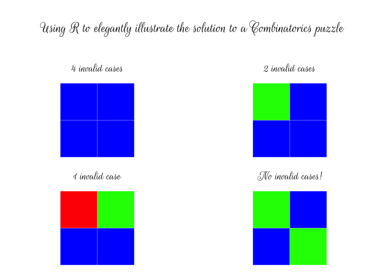
The first row confirms the count of $84$ valid cases, i.e., have no adjacency problem. Finally, because we can, and we love ggplot2, let’s generate 1 sample grid from each category of invalidity, so that we can visually inspect what we’ve been saying. The “4 invalid cases” has 4 pairs of blue, or 4 adjacencies, while the “No invalid cases!” plot is an example of how we can indeed color a graph, map, or a grid with 4 colors with no adjacent squares or “regions”, having the same color. Some notes on the code used – we plot the 4 examples using gridExtra. We’ll also use textGrob to attribute an overall title for the family of plots, using an elegant font from the Google library (“rouge script”). Click “Show the code” to see the details.

# Select first row of all groups
s <- invalid_data %>% group_by(invalid) %>% filter(row_number() == 1)

# Load necessary libraries for elegant visualizations
library(ggplot2)
library(grid)       # To ensure "textGrob" works
library(gridExtra)
library(showtext)   # For using custom fonts

# Load a font using showtext
font_add_google("Rouge Script", "rouge script")  # Example: Adding the "Lobster" font
showtext_auto()  # Automatically use showtext for all plots

# Create my color tibble (4x4)
sq <- s %>%
  mutate_all( ~ case_when(
    . == "b" ~ "blue",
    . == "g" ~ "green",
    . == "y" ~ "yellow",
    . == "r" ~ "red",
    TRUE ~ .  # Keep original value if it doesn't match
  ))

# Convert tibble to a matrix
color_matrix <- sq[, -5] %>% select(A, B, D, C) %>% as.matrix() # to match the coloring order of ggplot2

# Check the dimensions of the matrix
# Print(dim(color_matrix))  # Should be 4x4

# Function to create a plot based on a color vector and a title
create_plot <- function(colors, title) {
  df <- expand.grid(x = 0:1, y = 0:1)
  df$color <- colors
  
  ggplot(df, aes(x = x, y = y, fill = color)) +
    geom_tile(color = "white") +  # Change border color to white
    scale_fill_identity() +        # Use the colors as they are
    theme_minimal() +              # Use a minimal theme
    coord_fixed() +                # Keep aspect ratio
    labs(title = title) +          # Add the title
    theme(
      legend.position = "none",
      # Remove legend
      axis.title = element_blank(),
      # Suppress axis titles
      axis.text = element_blank(),
      # Suppress axis text
      axis.ticks = element_blank(),
      # Suppress axis ticks
      panel.grid = element_blank(),
      # Suppress grid lines
      plot.title = element_text(
        family = "rouge script",
        size = 16,
        hjust = 0.5
      )  # Use the custom font for the title
    )
}

# Create a vector of titles for each plot
titles <- c("4 invalid cases",
            "2 invalid cases",
            "1 invalid case",
            "No invalid cases!")

# Create a list of plots using the color matrix and titles
plots <- lapply(1:nrow(color_matrix), function(i) {
  create_plot(color_matrix[i, ], titles[i])
})

# Create the overall title using textGrob
overall_title <- textGrob(
  "Using R to elegantly illustrate the solution to a Combinatorics puzzle",
  gp = gpar(fontsize = 20, fontfamily = "rouge script")
)

# Create a spacer with appropriate height
spacer <- rectGrob(
  gp = gpar(fill = NA, col = NA),
  width = unit(1, "npc"),
  height = unit(0.5, "lines")
)

# Arrange the overall title and plots
grid.arrange(
  overall_title,
  spacer,
  arrangeGrob(grobs = plots, ncol = 2),
  ncol = 1,
  heights = c(1, 0.1, 4)
)

About the Author

Vidisha writes: “As a statistician and a data geek, I love solving puzzles of all kinds, with a particular fondness for combinatorial challenges. Recently, I tackled one in R using the dplyr package, which prompted me to think about the broader applications of R, not just as a powerful tool for solving puzzles for enthusiasts but also as an empowering way to teach high school mathematics. Moreover, R’s capabilities in data visualization can help learners grasp complex problems more intuitively, ultimately leading to a deeper understanding of their solutions.”