Packages used throughout the post
library(ggplot2)
library(grid)
library(dplyr)
library(msm)
library(gt)Most health care economics models are constructed from the perspective of a managed health care system such as those offered in Canada and several European countries, or from the perspective of some other third party such as an insurance company. Although the benefits of constructing models from the patient’s perspective have been discussed in the literature, see for example Ioannidis & Garber (2011) and Tai et al. (2016), few models have been published. Obvious reasons for this situation would include the privacy issues associated with obtaining patient specific data and the apparent lack of economic incentives to commit resources required to abstract individual patient trajectories from patient level data.
This post explores the hypothesis that detailed, data-driven, patient-specific models may not be necessary in order to achieve most of the benefits of a health economics model from the patients perspective. It present a lightweight, cohort model that captures the majority of the benefits to both physicians and patients that might result from a patient focused model.
The model is intended to be a proof of concept, a minimal viable model that may be useful to physicians both in deciding on treatment options and in informing patients about the potential outcomes and how they may experience these outcomes. To see how the medical literature may be helpful for this kind of modeling I explore the specific case of choosing between surgery and definitive radiation therapy for patients with stage II oral squamous cell carcinoma (OSCC).
Note that the model developed here is not being presented as a medical analysis. No medical experts have been consulted in its construction. It is merely being offered as an example of what could be done to build a health care economics model from a patient’s perspective with today’s modeling tools. Also note that I made significant use of Posit Assistant for the RStudio IDE configured with Claude Sonnet 4.6 which I found to be immensely helpful both for code construction and literature searches even though utility of the latter use was limited by the vexing proclivity of Claude to hallucinate.
The recovery of patients undergoing treatment OSCC, either surgery or radiation treatment, is conceived as a stochastic journey through various health states. The states visited, the sequence in which they are visited and the length of stay in each health state are modeled as random variables developing in in the framework of an eight=state, continuous-time Markov chain. Estimates of the transition probabilities among states and the mean time patients would remain in a state drive Markov chain. In the model below, these estimates are derived from the medical literature, however, it is conceivable that clinicians may feel comfortable in making their own estimates, or modifying the literature derived estimates according to their experience and their evaluations of their patients.
The next step uses the theory of continuous time Markov chains (CTMC) to construct a synthetic data set for a cohort of patients who vary in age and tumor size. The key insight here is that the synthetic data set is the underlying statistical model. Empirical survival curves and the time spent in each state and other useful quantities are then calculated from the synthetic data. The patient specific healthcare model is then constructed by estimating the utility of each health state to the patient. This is accomplished by constructing quality adjust life years (QALYs) based on EQ-5D values reported in the literature.
library(ggplot2)
library(grid)
library(dplyr)
library(msm)
library(gt)It is my understanding that although most patients wit stage II OSCC are treated with surgery there are times when surgery is either not possible or not preferable and the in these exceptional cases, radiation treatment is the primary alternative. The following state diagram is an attempt to abstract both the health states a patient will experience following treatment and the probable paths that will be taken among them. Eight states seemed to me to be the minimum number of states required to represent the complexities of treatment.
# library(ggplot2)
# library(grid)

BG <- "#F0F3F7"

# ── 1. Nodes ─────────────────────────────────────────────────────────────────
# Layout: left=initial treatment, center=adjuvant/NED, right=outcomes/death
nodes <- data.frame(
  id    = 1:8,
  label = c(
    "S1\nSurgery\n± Neck Dissection",
    "S2\nDefinitive\nRadiation",
    "S3\nPost-op\nSurveillance",
    "S4\nAdjuvant RT\n(PORT)",
    "S5\nAdjuvant\nChemoRT (POCRT)",
    "S6\nNED\n(Health)",
    "S7\nLocoregional\nRecurrence",
    "S8\nDeath"
  ),
  x    = c(1.5,  1.5,  4.5,  4.5,  4.5,  7.0,  9.5,  11.5),
  y    = c(8.5,  3.0,  9.5,  6.5,  3.5,  6.5,  7.5,   5.5),
  fill = c("#E67E22","#8E44AD","#F39C12","#2980B9","#16A085",
           "#27AE60","#C0392B","#2C3E50"),
  stringsAsFactors = FALSE
)

# ── 2. Edge definitions: from, to, label, curvature, nudge_x, nudge_y ────────
edge_defs <- list(
  # Surgery → downstream
  c(1, 3,  "No high-risk\nfeatures",    0.00,  0.10,  0.30),
  c(1, 4,  "High-risk:\nmargins/PNI/\nLVI/nodes",  0.10, -0.20,  0.20),
  c(1, 5,  "ECE/pos\nmargins",          0.18,  0.00, -0.30),
  c(1, 8,  "Peri-op\ndeath",           -0.22,  0.10, -0.20),
  # Definitive RT → downstream
  c(2, 6,  "NED",                       0.18,  0.00,  0.25),
  c(2, 7,  "Treatment\nfailure",        0.00,  0.00,  0.25),
  c(2, 8,  "Death",                     0.14, -0.10, -0.20),
  # Post-op Surveillance → downstream
  c(3, 6,  "",                          0.00,  0.10,  0.25),
  c(3, 7,  "",                          0.22,  0.20, -0.10),
  c(3, 8,  "",                         -0.18,  0.10, -0.18),
  # PORT → downstream
  c(4, 6,  "",                          0.00,  0.10,  0.25),
  c(4, 7,  "",                          0.12,  0.10,  0.18),
  c(4, 8,  "",                          0.14,  0.10, -0.18),
  # POCRT → downstream
  c(5, 6,  "",                          0.00,  0.10,  0.25),
  c(5, 7,  "",                          0.00,  0.10,  0.22),
  c(5, 8,  "",                          0.12,  0.10, -0.18),
  # NED → outcomes
  c(6, 7,  "LR recurrence",             0.00, -0.10,  0.25),
  c(6, 8,  "Death",                     0.18,  0.10, -0.14),
  # Locoregional Recurrence → outcomes
  c(7, 8,  "Death",                     0.00,  0.00,  0.25),
  c(7, 6,  "Salvage\nsuccess",         -0.28, -0.28,  0.00)
)

edges <- do.call(rbind, lapply(edge_defs, function(r) {
  data.frame(from=as.integer(r[[1]]), to=as.integer(r[[2]]),
             prob=r[[3]], curvature=as.numeric(r[[4]]),
             nudge_x=as.numeric(r[[5]]), nudge_y=as.numeric(r[[6]]),
             stringsAsFactors=FALSE)
}))

# Attach node coordinates
edges <- merge(edges, nodes[, c("id","x","y")], by.x="from", by.y="id", sort=FALSE)
names(edges)[names(edges)=="x"] <- "x0"; names(edges)[names(edges)=="y"] <- "y0"
edges <- merge(edges, nodes[, c("id","x","y","fill")], by.x="to", by.y="id", sort=FALSE)
names(edges)[names(edges)=="x"] <- "x1"; names(edges)[names(edges)=="y"] <- "y1"
names(edges)[names(edges)=="fill"] <- "dest_col"

# Shorten endpoints to node perimeter
NODE_R <- 0.58
shorten <- function(x0,y0,x1,y1,r) {
  dx<-x1-x0; dy<-y1-y0; d<-sqrt(dx^2+dy^2)
  list(xs=x0+dx*r/d, ys=y0+dy*r/d, xe=x1-dx*r/d, ye=y1-dy*r/d)
}
segs     <- Map(shorten, edges$x0, edges$y0, edges$x1, edges$y1, MoreArgs=list(r=NODE_R))
edges$xs <- sapply(segs,`[[`,"xs"); edges$ys <- sapply(segs,`[[`,"ys")
edges$xe <- sapply(segs,`[[`,"xe"); edges$ye <- sapply(segs,`[[`,"ye")
edges$lx <- (edges$xs+edges$xe)/2 + edges$nudge_x
edges$ly <- (edges$ys+edges$ye)/2 + edges$nudge_y

# ── 3. Build layers ───────────────────────────────────────────────────────────
arrow_layers <- lapply(seq_len(nrow(edges)), function(i) {
  e <- edges[i,,drop=FALSE]
  geom_curve(data=e, mapping=aes(x=xs,y=ys,xend=xe,yend=ye),
             curvature=e$curvature[[1]], colour=e$dest_col[[1]],
             linewidth=1.0, alpha=0.80,
             arrow=arrow(length=unit(9,"pt"), type="closed", ends="last"),
             show.legend=FALSE)
})

label_layers <- lapply(seq_len(nrow(edges)), function(i) {
  e <- edges[i,,drop=FALSE]
  if (nchar(trimws(e$prob[[1]])) == 0) return(NULL)
  geom_label(data=e, mapping=aes(x=lx,y=ly,label=prob),
             colour=e$dest_col[[1]], fill=BG, size=2.6, fontface="bold",
             label.size=0.22, label.r=unit(0.10,"lines"),
             label.padding=unit(0.15,"lines"), show.legend=FALSE)
})
label_layers <- Filter(Negate(is.null), label_layers)

# ── 4. Base plot ──────────────────────────────────────────────────────────────
base_plot <- ggplot() +
  theme_void(base_size=10) +
  theme(
    plot.background  = element_rect(fill=BG, colour=NA),
    panel.background = element_rect(fill=BG, colour=NA),
    plot.title  = element_text(family="serif", face="bold", size=16,
                               colour="#1A2535", hjust=0.5, margin=margin(b=4)),
    plot.subtitle = element_text(size=9, colour="#555555", hjust=0.5,
                                 margin=margin(b=10))
  ) +
  coord_fixed(xlim=c(0, 13), ylim=c(1.5, 11), clip="off") +
  labs(title="Stage II Oral Squamous Cell Carcinoma",
       subtitle="CTMC State Transition Diagram")

# ── 5. Assemble ───────────────────────────────────────────────────────────────
all_layers <- c(arrow_layers, label_layers,
  list(
    # Column labels
    annotate("text", x=1.5,  y=10.8, label="Initial\nTreatment",
             size=3.2, colour="#555", fontface="italic", hjust=0.5),
    annotate("text", x=4.5,  y=10.8, label="Post-surgical\nPathway",
             size=3.2, colour="#555", fontface="italic", hjust=0.5),
    annotate("text", x=7.0,  y=10.8, label="No Evidence\nof Disease",
             size=3.2, colour="#555", fontface="italic", hjust=0.5),
    annotate("text", x=9.5,  y=10.8, label="Disease\nProgression",
             size=3.2, colour="#555", fontface="italic", hjust=0.5),
    annotate("text", x=11.5, y=10.8, label="Absorbing\nState",
             size=3.2, colour="#555", fontface="italic", hjust=0.5),
    # Nodes
    geom_point(data=nodes, aes(x=x, y=y, colour=fill),
               size=28, show.legend=FALSE),
    scale_colour_identity(),
    geom_text(data=nodes, aes(x=x, y=y, label=label),
              colour="white", size=2.8, fontface="bold", lineheight=0.9),
    # Surgical candidate bracket
    annotate("segment", x=0.25, xend=0.25, y=2.2, yend=9.3,
             colour="#888", linewidth=0.5),
    annotate("segment", x=0.25, xend=0.45, y=9.3, yend=9.3,
             colour="#888", linewidth=0.5),
    annotate("segment", x=0.25, xend=0.45, y=2.2, yend=2.2,
             colour="#888", linewidth=0.5),
    annotate("text", x=0.0, y=5.75, label="Surgical\ncandidate?\nYes ↑\nNo ↓",
             size=2.8, colour="#666", hjust=0.5, lineheight=0.9)
  )
)

Reduce("+", all_layers, init=base_plot)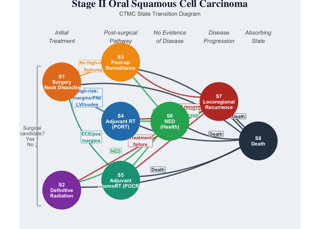
| State | Label | Role |
|---|---|---|
| S1 | Surgery | Initial surgical treatment (days–weeks) |
| S2 | DefinitiveRT | Non-surgical candidates; 6–7 week RT course |
| S3 | PostOpSurveillance | Surgery, no high-risk pathological features |
| S4 | AdjuvantRT (PORT) | High-risk: margins, PNI, LVI, multiple nodes |
| S5 | AdjuvantChemoRT (POCRT) | Highest-risk: ECE or positive margins |
| S6 | NED | No evidence of disease; long-term surveillance |
| S7 | LR Recurrence | Locoregional recurrence at primary or nodes |
| S8 | Death | Absorbing state |
This section builds a synthetic patient cohort for Stage II (T2 N0 M0) oral squamous cell carcinoma using a continuous-time Markov chain (CTMC). The first code block sets up of the simulation by defining the covariates: patient age and tumor size. Mean patient age is set at 62 years old. Tumor size ranges from tumor 2-4 cm, DOI 5-10 mm
set.seed(6413)

N_PATIENTS <- 1000
MAX_TIME   <- 60      # months (5-year follow-up)
obs_base   <- c(0, 1, 2, 3, 6, 9, 12, 18, 24, 36, 48, 60)

state_labels_ii <- c(
  "Surgery", "DefinitiveRT", "PostOpSurveillance",
  "AdjuvantRT_PORT", "AdjuvantChemoRT_POCRT",
  "NED", "LR_Recurrence", "Death"
)

# ── Patient covariates ────────────────────────────────────────────────────────
# Stage II OSCC (T2 N0 M0): tumor 2-4 cm, DOI 5-10 mm
age           <- as.integer(round(rnorm(N_PATIENTS, mean = 62, sd = 11)))
age           <- pmax(32L, pmin(85L, age))
tumor_size_cm <- round(runif(N_PATIENTS, 2.0, 4.0), 1)
DOI_mm        <- round(runif(N_PATIENTS, 5.0, 10.0), 1)

# Surgical candidacy: logistic model, ~78% surgery at age 60
surgery_prob <- plogis(1.5 - 0.04 * (age - 60))
treatment <- ifelse(runif(N_PATIENTS) < surgery_prob, "Surgery", "DefinitiveRT")The simulation is driven by two sets of clinician-interpret able inputs that are entered at the beginning of this section of code:
jump_P[i,j]: given that a patient leaves state i, the probability they transition directly to state j.mean_sojourn[i]: the average time (months) a patient spends in state i before transitioning.The jump chain may be thought of as an embedded discrete time Markov chain that gives the probabilities of which state the chain will jump to next when it is time to jump. The sojourn times are inverted to obtain the transition rates. The values for these parameters have been derived from the literature, however, the model has been set up so that they can be easily changed if the physician thinks that a particular class of patients would be better represented by other values. The justifications for the default values for the parameters driving the model are provided in the comments in the code and in the references below.
# == CLINICIAN INPUTS ==========================================================
#
# jump_P[i, j]  : probability of moving to state j *given* a transition occurs
#                 from state i.  Rows must sum to 1 for states 1-7.
#
# mean_sojourn  : average time (months) in each transient state.
#
# Together these fully specify the CTMC generator:
#   Q[i, j] = jump_P[i, j] / mean_sojourn[i]   (off-diagonal)
# All downstream simulation code derives Q_base automatically from these inputs.

# ── Jump chain transition probabilities ───────────────────────────────────────


jump_P <- matrix(0, 8, 8,
  dimnames = list(paste0("S", 1:8), paste0("S", 1:8)))

# S1 (Surgery) -> {S3=no high-risk, S4=PORT, S5=POCRT, S8=peri-op death}
# ~20-30% high-risk features -> PORT (Tassone et al. 2023, NCDB n=53,503; DOI:10.1002/ohn.205)
# ~10-15% ECE/pos margins -> POCRT; peri-operative mortality ~1-2% (Nathan et al. 2025, NSQIP n=866; DOI:10.18203/issn.2454-5929.ijohns20252980)
# NB: S8 revised from 0.05 to 0.015 — the original 5% exceeded the literature range of 1-2%;
# freed mass (0.035) reallocated to S3 (residual no-adjuvant group), S4 and S5 unchanged.
jump_P[1, c(3, 4, 5, 8)] <- c(0.585, 0.25, 0.15, 0.015)

# S2 (DefinitiveRT) -> {S6=NED, S7=treatment failure, S8=death}
# Definitive RT alone locoregional control ~65% for T2N0M0 (Dana-Farber Group 2011 PMID 21531515, 2-yr LRC 64%; Studer et al. 2007 T2-4 LC ~50-60%)
jump_P[2, c(6, 7, 8)] <- c(0.65, 0.28, 0.07)

# S3 (PostOpSurveillance) -> {S6=NED, S7=LR recurrence, S8=death}
# 5-yr LR recurrence ~12-18% after margin-negative R0 surgery alone (Ord 2006 15.5%; Luryi 2014 NCDB early-stage series)
jump_P[3, c(6, 7, 8)] <- c(0.74, 0.18, 0.08)

# S4 (PORT) -> {S6=NED, S7=LR recurrence, S8=death}
# After PORT, 3-yr OS ~71% (95% CI 67-75%) in adjuvant PORT cohort (Hosni et al. 2019, PMID: 30244160)
jump_P[4, c(6, 7, 8)] <- c(0.67, 0.23, 0.10)

# S5 (POCRT) -> {S6=NED, S7=LR recurrence, S8=death}
# After POCRT, locoregional control ~60%; Stage II mortality revised down to 10% (Bernier 2004, Cooper 2004; Stage II subgroup)
jump_P[5, c(6, 7, 8)] <- c(0.60, 0.30, 0.10)

# S6 (NED) -> {S7=LR recurrence, S8=death}
# ~75% leave NED via recurrence vs other-cause death (SEER Stage II split)
jump_P[6, c(7, 8)] <- c(0.75, 0.25)

# S7 (LR Recurrence) -> {S6=salvage success, S8=death}
# Salvage success 0.43 / mortality 0.57: Lee et al. 2024 pooled 5-yr OS = 43% (n=2069); revised from c(0.25, 0.75) — previous value over-estimated post-recurrence mortality
jump_P[7, c(6, 8)] <- c(0.43, 0.57)

# ── Mean sojourn times (months) ───────────────────────────────────────────────
mean_sojourn <- c(
  1.5,   # S1  Surgery: weighted mean accounting for real-world S-PORT delays ~8-9 wks (Correia 2026; Dayan 2023; Graboyes 2017)
  3.0,   # S2  DefinitiveRT: RT course (1.5 mo) + post-RT response assessment window >=12 wks (NCCN HNC Guidelines; Mehanna et al. 2016 [PET-NECK] PMID 26958921)
  22.0,  # S3  PostOpSurveillance: weighted mean to event (NED@24mo x0.74 + recur@18mo x0.18 + death@14mo x0.08) = 22 mo (Blatt 2022; Brands 2019; Ord 2006)
  3.0,   # S4  PORT: ~6-week adjuvant RT + recovery — supported, unchanged
  4.0,   # S5  POCRT: ~6-week concurrent chemoRT + extended recovery — supported, unchanged
  120.0, # S6  NED: calibrated to SEER ~20% 5-yr recurrence; exit rate 0.0083/mo -> mean 120 mo (SEER localized OCC; Brands 2019; Luryi 2014)
  12.5,  # S7  LR Recurrence: median OS ~12-18 mo all-comers (Liu 2007; Contrera 2022) — within supported range, unchanged
  NA     # S8  Death (absorbing)
)
names(mean_sojourn) <- paste0("S", 1:8)

# == END CLINICIAN INPUTS ======================================================

# ── Derive Q_base from clinician inputs ───────────────────────────────────────
# Q[i,j] = jump_P[i,j] / mean_sojourn[i]
Q_base <- matrix(0, 8, 8)
for (i in 1:7) {
  for (j in which(jump_P[i, ] > 0)) {
    Q_base[i, j] <- jump_P[i, j] / mean_sojourn[i]
  }
}
diag(Q_base) <- -rowSums(Q_base)as.data.frame(jump_P) S1 S2 S3 S4 S5 S6 S7 S8
S1 0 0 0.585 0.25 0.15 0.00 0.00 0.015
S2 0 0 0.000 0.00 0.00 0.65 0.28 0.070
S3 0 0 0.000 0.00 0.00 0.74 0.18 0.080
S4 0 0 0.000 0.00 0.00 0.67 0.23 0.100
S5 0 0 0.000 0.00 0.00 0.60 0.30 0.100
S6 0 0 0.000 0.00 0.00 0.00 0.75 0.250
S7 0 0 0.000 0.00 0.00 0.43 0.00 0.570
S8 0 0 0.000 0.00 0.00 0.00 0.00 0.000data.frame(
#State = paste0("S", 1:7),
Label = state_labels_ii[1:7],
Mean_sojourn = mean_sojourn[1:7],
Total_rate = round(-diag(Q_base)[1:7], 4)
) Label Mean_sojourn Total_rate
S1 Surgery 1.5 0.6667
S2 DefinitiveRT 3.0 0.3333
S3 PostOpSurveillance 22.0 0.0455
S4 AdjuvantRT_PORT 3.0 0.3333
S5 AdjuvantChemoRT_POCRT 4.0 0.2500
S6 NED 120.0 0.0083
S7 LR_Recurrence 12.5 0.0800This code block constructs the synthetic data and prints out the first few rows of the synthetic data set.
# ── Patient-specific Q (covariates scale recurrence & mortality rates) ─────────
make_Q <- function(age_i, size_i) {
  Q <- Q_base
  age_eff  <- exp(0.025 * (age_i  - 60))   # older  -> higher mortality
  size_eff <- exp(0.180 * (size_i -  3.0))  # larger -> higher recurrence
  Q[3, 7] <- Q_base[3, 7] * size_eff        # PostOpSurv -> LR Recurrence
  Q[6, 7] <- Q_base[6, 7] * size_eff * age_eff
  Q[6, 8] <- Q_base[6, 8] * age_eff
  Q[7, 8] <- Q_base[7, 8] * age_eff
  diag(Q) <- 0
  diag(Q) <- -rowSums(Q)
  Q
}

# ── Simulate one patient's full CTMC path ─────────────────────────────────────
sim_ctmc <- function(init_s, Q_i, max_t) {
  t_vec <- 0; s_vec <- init_s; s <- init_s; t <- 0
  while (t < max_t && s != 8L) {
    total_rate <- -Q_i[s, s]
    if (total_rate == 0) break
    t <- t + rexp(1L, total_rate)
    if (t > max_t) break
    probs    <- pmax(Q_i[s, ], 0)
    probs[s] <- 0
    s        <- sample.int(8L, 1L, prob = probs)
    t_vec    <- c(t_vec, t); s_vec <- c(s_vec, s)
  }
  list(times = t_vec, states = s_vec)
}

# State at a given observation time (last known state)
state_at <- function(traj, obs_t) {
  traj$states[max(which(traj$times <= obs_t))]
}

# ── Generate panel data ────────────────────────────────────────────────────────
records <- vector("list", N_PATIENTS)

for (i in seq_len(N_PATIENTS)) {
  init_s  <- if (treatment[i] == "Surgery") 1L else 2L
  Q_i     <- make_Q(age[i], tumor_size_cm[i])
  traj    <- sim_ctmc(init_s, Q_i, MAX_TIME)

  jitter  <- c(0, runif(length(obs_base) - 1L, -0.5, 0.5))
  obs_t   <- sort(unique(pmax(0, obs_base + jitter)))

  death_t <- if (8L %in% traj$states)
    traj$times[which(traj$states == 8L)[1L]]
  else Inf

  obs_t <- obs_t[obs_t < death_t]
  if (is.finite(death_t) && death_t <= MAX_TIME)
    obs_t <- c(obs_t, death_t)

  obs_s <- sapply(obs_t, state_at, traj = traj)

  records[[i]] <- data.frame(
    id            = i,
    time          = round(obs_t, 2),
    state         = obs_s,
    age           = age[i],
    tumor_size_cm = tumor_size_cm[i],
    DOI_mm        = DOI_mm[i],
    treatment     = treatment[i],
    stringsAsFactors = FALSE
  )
}

oscc2_data <- do.call(rbind, records)
rownames(oscc2_data) <- NULL
oscc2_data$state_label <- state_labels_ii[oscc2_data$state]

# Save synthetic data
write.csv(oscc2_data, "OSCC_HE_Synthetic_Data.csv", row.names = FALSE)

# First 10 rows
head(oscc2_data, 10)
id time state age tumor_size_cm DOI_mm treatment state_label
1 1 0.00 1 59 2.2 7.8 Surgery Surgery
2 1 1.38 1 59 2.2 7.8 Surgery Surgery
3 1 1.82 1 59 2.2 7.8 Surgery Surgery
4 1 3.01 1 59 2.2 7.8 Surgery Surgery
5 1 6.04 3 59 2.2 7.8 Surgery PostOpSurveillance
6 1 8.50 3 59 2.2 7.8 Surgery PostOpSurveillance
7 1 11.61 3 59 2.2 7.8 Surgery PostOpSurveillance
8 1 17.91 3 59 2.2 7.8 Surgery PostOpSurveillance
9 1 24.01 3 59 2.2 7.8 Surgery PostOpSurveillance
10 1 35.86 6 59 2.2 7.8 Surgery NEDNote that two covariates: age of patient and tumor size are included in the data ane encoded in the make_Q function used to create the synthetic data as follows:
age_eff <- exp(0.025 * (age_i - 60)) # older -> higher mortalitysize_eff <- exp(0.180 * (size_i - 3.0)) # larger -> higher recurrenceThis table shows some of the meta-data describing the synthetic data set.
# Collect components for footnotes
trt_counts <- table(treatment)
died <- oscc2_data |>
  dplyr::filter(state == 8) |>
  dplyr::distinct(id) |>
  nrow()

# Main table: state visit counts
as.data.frame(table(State = oscc2_data$state_label)) |>
  gt() |>
  tab_options(table.font.size = px(12)) |>
  cols_label(State = "State", Freq = "Observations") |>
  tab_source_note(md(paste0(
    "**Dataset:** ", nrow(oscc2_data), " observations; ",
    N_PATIENTS, " patients"
  ))) |>
  tab_source_note(md(paste0(
    "**Treatment:** Surgery = ", trt_counts["Surgery"],
    "; DefinitiveRT = ", trt_counts["DefinitiveRT"]
  ))) |>
  tab_source_note(md(paste0(
    "**Mortality:** ", died, " / ", N_PATIENTS,
    " patients reached Death (",
    round(100 * died / N_PATIENTS, 1), "%)"
)))| State | Observations |
|---|---|
| AdjuvantChemoRT_POCRT | 228 |
| AdjuvantRT_PORT | 333 |
| Death | 370 |
| DefinitiveRT | 570 |
| LR_Recurrence | 767 |
| NED | 4407 |
| PostOpSurveillance | 2381 |
| Surgery | 1578 |
| Dataset: 10634 observations; 1000 patients | |
| Treatment: Surgery = 794; DefinitiveRT = 206 | |
| Mortality: 370 / 1000 patients reached Death (37%) | |
This data frame shows the complete trajectory of sates visited for the first synthetic patient.
oscc2_data[oscc2_data$id == 1,
           c("id", "time", "state", "state_label", "treatment",
             "age", "tumor_size_cm", "DOI_mm")]
id time state state_label treatment age tumor_size_cm DOI_mm
1 1 0.00 1 Surgery Surgery 59 2.2 7.8
2 1 1.38 1 Surgery Surgery 59 2.2 7.8
3 1 1.82 1 Surgery Surgery 59 2.2 7.8
4 1 3.01 1 Surgery Surgery 59 2.2 7.8
5 1 6.04 3 PostOpSurveillance Surgery 59 2.2 7.8
6 1 8.50 3 PostOpSurveillance Surgery 59 2.2 7.8
7 1 11.61 3 PostOpSurveillance Surgery 59 2.2 7.8
8 1 17.91 3 PostOpSurveillance Surgery 59 2.2 7.8
9 1 24.01 3 PostOpSurveillance Surgery 59 2.2 7.8
10 1 35.86 6 NED Surgery 59 2.2 7.8
11 1 47.91 6 NED Surgery 59 2.2 7.8
12 1 59.89 6 NED Surgery 59 2.2 7.8This next plot shows overall survival (Kaplan-Meier) curves for patients in both treatment arms. Note that surgery exhibits a slightly better overall survival curve (Approximately 73% vs approximately 65% at 5 years). However, both curves show very good five year survival probabilities.
Three external benchmark points are overlaid on the Kaplan–Meier curves as filled diamonds.
While not validating the survival curves, the benchmark points indicate that they are a plausible starting point for analysis.
library(survival)
library(survminer)

# One row per patient: time to death or end of follow-up
km_input <- oscc2_data |>
  dplyr::group_by(id, treatment) |>
  dplyr::summarise(
    time  = max(time),
    event = as.integer(any(state == 8)),
    .groups = "drop"
  )

km_fit_2arm <- survfit(Surv(time, event) ~ treatment, data = km_input)

km_plot <- ggsurvplot(
  km_fit_2arm,
  data        = km_input,
  conf.int    = FALSE,
  risk.table  = TRUE,
  palette     = c("#D55E00", "#0072B2"),   # DefinitiveRT=orange, Surgery=blue (alphabetical strata order)
  legend.labs = c("Definitive RT", "Surgery"),
  xlab        = "Time (months)",
  ylab        = "Survival probability",
  title       = "Overall Survival — Stage II OSCC",
  ylim        = c(0.25, 1),
  ggtheme     = theme_bw()
)

# Overlay external benchmark points (diamonds) on the KM plot
km_plot$plot <- km_plot$plot +
  annotate("point", x = 60, y = 0.77, shape = 23, size = 4,
           fill = "#0072B2", color = "black") +
  annotate("text",  x = 60, y = 0.77,
           label = "Siegel 2024\n(SEER ~77%)", vjust = -0.35, hjust = 0.5, size = 2.8) +
  annotate("point", x = 36, y = 0.71, shape = 23, size = 4,
           fill = "#0072B2", color = "black") +
  annotate("text",  x = 36, y = 0.71,
           label = "Hosni 2019\n(71% at 3 yr)", vjust = -0.35, hjust = 0.5, size = 2.8) +
  annotate("point", x = 24, y = 0.63, shape = 23, size = 4,
           fill = "#D55E00", color = "black") +
  annotate("text",  x = 24, y = 0.63,
           label = "Sher 2011\n(63% at 2 yr)", vjust = 1.6, hjust = 0.5, size = 2.8)

km_plot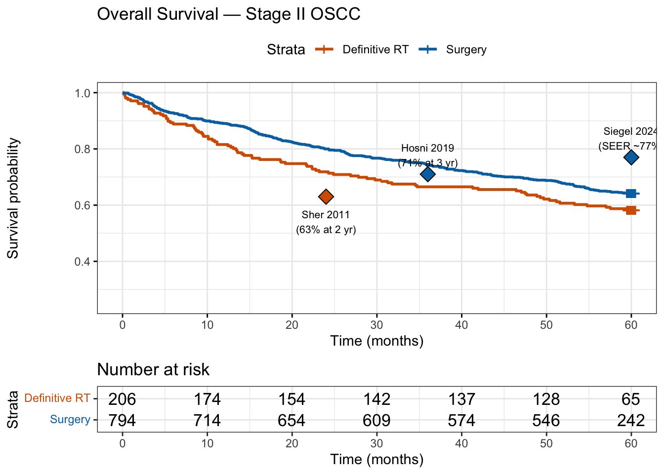
This next panel of plots show the overall survival broken out by the covariates age and tumor size. Each panel indicates the four possible values of the covariates.
library(broom)
library(ggplot2)
library(dplyr)

# ── One row per patient with covariate categories ─────────────────────────────
# Age split at 62 (simulation mean); tumour size split at 3 cm (Stage II midpoint)
km_cov <- oscc2_data |>
  dplyr::group_by(id, treatment) |>
  dplyr::summarise(
    time          = max(time),
    event         = as.integer(any(state == 8)),
    age           = first(age),
    tumor_size_cm = first(tumor_size_cm),
    .groups       = "drop"
  ) |>
  dplyr::mutate(
    age_grp  = factor(ifelse(age  < 62,  "Age < 62",   "Age ≥ 62"),
                      levels = c("Age < 62", "Age ≥ 62")),
    size_grp = factor(ifelse(tumor_size_cm < 3.0, "Tumour < 3 cm", "Tumour ≥ 3 cm"),
                      levels = c("Tumour < 3 cm", "Tumour ≥ 3 cm")),
    covariate_group = factor(
      interaction(age_grp, size_grp, sep = ", "),
      levels = c(
        "Age < 62, Tumour < 3 cm",
        "Age < 62, Tumour ≥ 3 cm",
        "Age ≥ 62, Tumour < 3 cm",
        "Age ≥ 62, Tumour ≥ 3 cm"
      )
    )
  )

pal4  <- c("#2166AC", "#92C5DE", "#D6604D", "#B2182B")
labs4 <- c("Age < 62, Tumour < 3 cm",
           "Age < 62, Tumour ≥ 3 cm",
           "Age ≥ 62, Tumour < 3 cm",
           "Age ≥ 62, Tumour ≥ 3 cm")

# ── Tidy survival estimates per arm ──────────────────────────────────────────
tidy_arm <- function(arm, data) {
  df  <- dplyr::filter(data, treatment == arm)
  fit <- survfit(Surv(time, event) ~ covariate_group, data = df)
  broom::tidy(fit, conf.int = FALSE) |>
    dplyr::mutate(
      treatment = arm,
      covariate_group = factor(
        sub("covariate_group=", "", strata),
        levels = levels(data$covariate_group)
      )
    )
}

surv_tidy <- dplyr::bind_rows(
  tidy_arm("Surgery",      km_cov),
  tidy_arm("DefinitiveRT", km_cov)
) |>
  dplyr::mutate(treatment = factor(treatment,
    levels = c("Surgery", "DefinitiveRT"),
    labels = c("Surgery Arm", "Definitive RT Arm")))

# ── Two-panel KM plot ─────────────────────────────────────────────────────────
ggplot(surv_tidy, aes(x = time, y = estimate,
                      colour = covariate_group,
                      group  = covariate_group)) +
  geom_step(linewidth = 0.8) +
  facet_wrap(~treatment, ncol = 2) +
  scale_colour_manual(values = pal4, labels = labs4) +
  scale_y_continuous(labels = scales::percent_format(accuracy = 1),
                     limits = c(0, 1), breaks = seq(0, 1, 0.25)) +
  scale_x_continuous(limits = c(0, 60), breaks = seq(0, 60, 12)) +
  labs(
    x      = "Time (months)",
    y      = "Survival probability",
    colour = "Age / Tumour Size",
    title  = "Overall Survival by Age and Tumour Size — Stage II OSCC"
  ) +
  theme_bw(base_size = 11) +
  theme(
    legend.position  = "bottom",
    legend.direction = "horizontal",
    legend.text      = element_text(size = 9),
    legend.title     = element_text(size = 10, face = "bold"),
    strip.text       = element_text(size = 11, face = "bold"),
    plot.title       = element_text(size = 12, face = "bold")
  ) +
  guides(colour = guide_legend(nrow = 2, byrow = TRUE))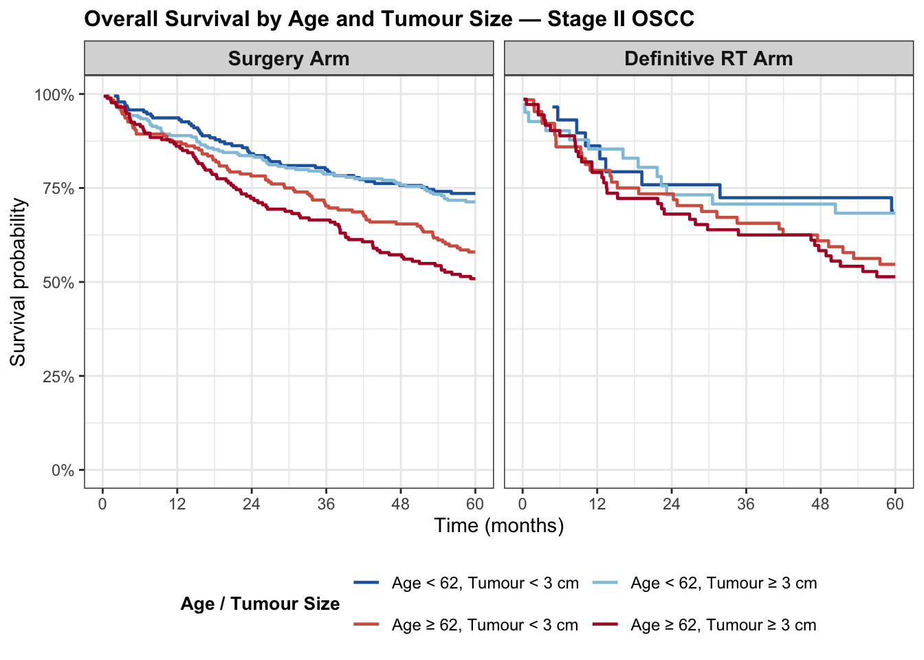
Surgery arm (n = 794): age is the dominant predictor of survival. The youngest, smallest-tumour subgroup (Age < 62, Tumour < 3 cm; dark blue) reaches 74% at 5 years, while the youngest with larger tumours (Age < 62, Tumour ≥ 3 cm; light blue) reaches 71% Among older patients (Age ≥ 62), those with smaller tumours (Tumour < 3 cm; orange) fare worst at 58%, while those with larger tumours (dark red) reach 51%. Even if these counter intuitive orderings are due to sampling variation and not a more fundamental underlying cause they may indicate a limitation of the this particular synthetic data set.
Definitive RT arm (n = 206): the four subgroups together contain only 206 patients, yielding wide confidence bands and coarse staircase steps; point estimates (69%, 68%, 55%, 51% for the dark-blue, light-blue, orange, and dark-red subgroups respectively) should be interpreted with caution. The broad pattern mirrors the Surgery arm in that older age is associated with lower survival, but the small-n instability makes subgroup comparisons across treatment arms unreliable.
Progression-free survival (PFS) is defined here as the time from treatment start to the first occurrence of either locoregional recurrence (S7) or death (S8), whichever comes first. Patients who reached neither endpoint by month 60 are censored at their last observed time.
library(survival)
library(survminer)

# ── Build per-patient PFS endpoint ───────────────────────────────────────────
# Event = first entry into LR_Recurrence (state 7) or Death (state 8)
pfs_events <- oscc2_data |>
  dplyr::filter(state %in% c(7L, 8L)) |>
  dplyr::group_by(id) |>
  dplyr::slice_min(time, n = 1, with_ties = FALSE) |>
  dplyr::ungroup() |>
  dplyr::select(id, pfs_time = time, pfs_event_type = state_label)

last_obs <- oscc2_data |>
  dplyr::group_by(id) |>
  dplyr::slice_max(time, n = 1, with_ties = FALSE) |>
  dplyr::ungroup() |>
  dplyr::select(id, last_time = time, treatment)

pfs_df <- last_obs |>
  dplyr::left_join(pfs_events, by = "id") |>
  dplyr::mutate(
    pfs_time  = dplyr::coalesce(pfs_time, last_time),
    pfs_event = as.integer(!is.na(pfs_event_type))
  )

# ── Fit KM curves ─────────────────────────────────────────────────────────────
km_pfs <- survfit(Surv(pfs_time, pfs_event) ~ treatment, data = pfs_df)
km_pfs_named <- km_pfs
names(km_pfs_named$strata) <- c("Definitive RT", "Surgery")

# ── Plot with at-risk table ───────────────────────────────────────────────────
ggsurvplot(
  km_pfs_named,
  data              = pfs_df,
  palette           = c("#D55E00", "#0072B2"),
  conf.int          = TRUE,
  conf.int.alpha    = 0.15,
  size              = 0.9,
  risk.table        = TRUE,
  risk.table.col    = "strata",
  risk.table.height = 0.25,
  tables.theme      = theme_cleantable(),
  xlab              = "Time (months)",
  ylab              = "Progression-free probability",
  title             = "Progression-Free Survival — Stage II OSCC",
  legend.title      = "Treatment",
  legend.labs       = c("Definitive RT", "Surgery"),
  legend            = "bottom",
  surv.median.line  = "hv",
  break.time.by     = 12,
  xlim              = c(0, 60),
  ylim              = c(0, 1),
  ggtheme           = theme_minimal(base_size = 13),
  fontsize          = 4
)
tbl_fun <- function(s) {
  data.frame(
    Treatment = as.character(s$strata),
    Time      = s$time,
    PFS       = round(s$surv,  3),
    Lower95   = round(s$lower, 3),
    Upper95   = round(s$upper, 3)
  )
}
tbl_fun(summary(km_pfs_named, times = c(12, 24, 36, 48, 60))) |>
  knitr::kable(
    col.names = c("Treatment", "Month", "PFS", "95% CI lower", "95% CI upper"),
    caption   = "Kaplan-Meier PFS estimates at annual checkpoints"
)| Treatment | Month | PFS | 95% CI lower | 95% CI upper |
|---|---|---|---|---|
| Definitive RT | 12 | 0.631 | 0.569 | 0.701 |
| Definitive RT | 24 | 0.573 | 0.509 | 0.645 |
| Definitive RT | 36 | 0.544 | 0.480 | 0.616 |
| Definitive RT | 48 | 0.519 | 0.455 | 0.592 |
| Definitive RT | 60 | 0.449 | 0.386 | 0.523 |
| Surgery | 12 | 0.783 | 0.755 | 0.813 |
| Surgery | 24 | 0.683 | 0.651 | 0.716 |
| Surgery | 36 | 0.617 | 0.584 | 0.652 |
| Surgery | 48 | 0.564 | 0.531 | 0.600 |
| Surgery | 60 | 0.511 | 0.477 | 0.548 |
The total times that patients are expected to spend in each state over a 60-month horizon drive the economics analysis. The ability to make this calculation is the primary motivation for modeling the treatment regimen as a continuous time Markov chain.
library(expm)

# Adapted from plot_msm_state_occupancy() (Breast_Cancer_v3.qmd).
# Accepts Q_base directly instead of a fitted msm model, and accepts
# a start_state argument so the two treatment arms can be compared.
plot_state_occupancy <- function(Q,
                                 start_state  = 1,
                                 tmax         = 60,
                                 tstep        = 0.5,
                                 state_labels = NULL,
                                 title        = "State Occupancy Probabilities") {
  n_states    <- nrow(Q)
  start_probs <- rep(0, n_states)
  start_probs[start_state] <- 1
  time <- seq(0, tmax, by = tstep)

  occ <- matrix(NA, nrow = length(time), ncol = n_states)
  colnames(occ) <- paste0("S", seq_len(n_states))
  for (i in seq_along(time))
    occ[i, ] <- start_probs %*% expm(Q * time[i])

  df_long <- as.data.frame(occ) |>
    dplyr::mutate(time = time) |>
    tidyr::pivot_longer(-time, names_to = "state", values_to = "prob")

  if (!is.null(state_labels))
    df_long$state <- factor(df_long$state,
      levels = paste0("S", seq_len(n_states)),
      labels = state_labels)

  ggplot(df_long, aes(x = time, y = prob, colour = state)) +
    geom_line(linewidth = 1.0) +
    labs(x = "Time (months)", y = "Probability",
         title = title, colour = "State") +
    theme_bw(base_size = 12)
}

# Expected time in each state: trapezoid integral of P(t) over 0-60 months
compute_state_time <- function(Q, start_state, tmax = 60, tstep = 0.5) {
  n_states    <- nrow(Q)
  start_probs <- rep(0, n_states)
  start_probs[start_state] <- 1
  time <- seq(0, tmax, by = tstep)
  occ  <- matrix(NA, nrow = length(time), ncol = n_states)
  for (i in seq_along(time))
    occ[i, ] <- start_probs %*% expm(Q * time[i])
  apply(occ, 2, function(p)
    sum(diff(time) * (p[-1] + p[-length(p)]) / 2))
}time_surg <- compute_state_time(Q_base, start_state = 1)
time_def <- compute_state_time(Q_base, start_state = 2)
data.frame(
State = paste0("S", 1:8),
Label = state_labels_ii,
Surgery_mo = round(time_surg, 2),
DefRT_mo = round(time_def, 2)
) State Label Surgery_mo DefRT_mo
1 S1 Surgery 1.51 0.00
2 S2 DefinitiveRT 0.00 3.01
3 S3 PostOpSurveillance 11.96 0.00
4 S4 AdjuvantRT_PORT 0.75 0.00
5 S5 AdjuvantChemoRT_POCRT 0.60 0.00
6 S6 NED 28.83 35.54
7 S7 LR_Recurrence 4.09 5.67
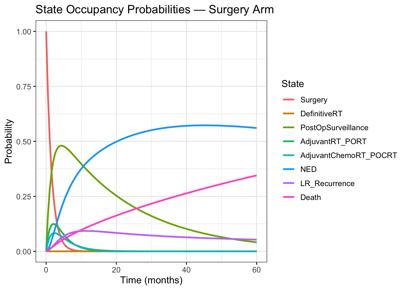
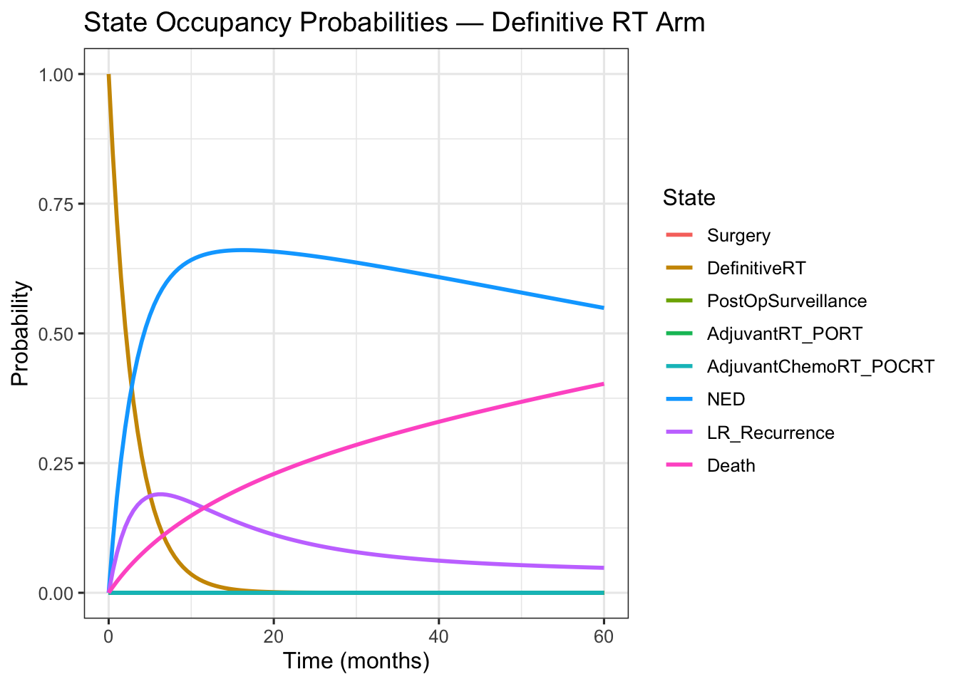
8 S8 Death 12.26 15.78The state occupancy plots show the probability of being in each state as time progresses. For both plots, focusing on a particular time point gives a gives an estimate of a patient’s probable health state.
plot_state_occupancy(
  Q            = Q_base,
  start_state  = 1,
  state_labels = state_labels_ii,
  title        = "State Occupancy Probabilities — Surgery Arm"
)
plot_state_occupancy(
  Q            = Q_base,
  start_state  = 2,
  state_labels = state_labels_ii,
  title        = "State Occupancy Probabilities — Definitive RT Arm"
)
The health Economics model presented uses QALYs calculated with with EQ-5D utilities. Although these utilities are abstractions they do provide a measure, however imperfect, of how patients treated for OSCC have rated the ensemble of experiences related to each possible health state.
The model does not to calculate financial costs for the following reasons:
A Quality-Adjusted Life Year (QALY) combines the quantity and quality of life into a single metric. One QALY represents one year lived in perfect health; a year spent in a health state with diminished quality counts for less than one QALY in proportion to that state’s utility weight.
In this model, QALYs are calculated in three steps:
Assign utility weights: Each of the eight health states is assigned an EQ-5D utility value between 0 (death) and 1 (perfect health), drawn from peer-reviewed literature on head-and-neck cancer patients.
Estimate time in each state: The continuous-time Markov chain (CTMC) simulation provides the expected number of months the cohort spends in each state over a 60-month horizon, separately for the Surgery arm and the Definitive Radiation Therapy arm.
Compute utility-weighted life years: For each state, the time (in months) is multiplied by its utility weight and the products are summed across all states. Dividing by 12 converts the result to years:
\[ \text{Total QALYs} = \frac{1}{12} \sum_{i=1}^{8} \text{time}_i \times u_i \]
where \(\text{time}_i\) is the expected months in state \(i\) and \(u_i\) is its EQ-5D utility. The two treatment arms are evaluated on the same 60-month horizon, allowing a direct QALY comparison from the patient’s perspective.
Health state utility values map each model state to a preference-based quality-of-life weight on the 0–1 scale (0 = death, 1 = perfect health). The weights below are EQ-5D-based defaults drawn from the published literature. S6 (NED) carries the highest utility among living states and serves as the reference; a NED-normalized column (NED = 1.00) is included for sensitivity work.
The sources for the utility values are provided as comments in the code below. Complete references are provided in the Reference section at the end.
# Health state utility values (EQ-5D scale, 0 = death, 1 = perfect health).
# S6 (NED) is the reference (highest) living state.
# Sources:
# S1 de Almeida et al. 2014; Noel et al. 2015
# S2 Sprave et al. 2022 (during-RT EQ-5D ~0.83, n=366); Truong/RTOG 0522 2017 retained for S5
# S3 Govers et al. 2016
# S4 Sprave et al. 2022 (during-RT EQ-5D ~0.83, n=366); Govers et al. 2016
# S5 Truong et al. / RTOG 0522 2017 (primary); Sprave et al. 2022 adjuvant CRT data support ~0.83 but POCRT toxicity justifies retaining 0.775 — see inline note
# S6 Noel et al. 2015 (reference state)
# S7 Meregaglia & Cairns 2017 (systematic review confirming evidence gap; only patient EQ-5D for recurrence found is median 0.70, del Barco et al. 2016, palliative/metastatic context); 0.55 is modeller's assumption
# S8 Convention (absorbing state)
utility <- c(
  S1 = 0.60,   # Surgery: acute peri-operative period
  S2 = 0.83,   # DefinitiveRT: during 6-7 week RT course (Sprave et al. 2022, mean EQ-5D at RT completion = 0.830, n=366)
  S3 = 0.72,   # PostOpSurveillance: recovery phase
  S4 = 0.83,   # PORT: adjuvant RT toxicity (Sprave et al. 2022, mean EQ-5D at RT completion = 0.830, n=366)
  S5 = 0.775, # POCRT: concurrent chemoRT (revised from 0.60). Primary source: Truong/RTOG 0522 3-month EQ-5D proxy (CIS arm 0.78, CET/CIS arm 0.77); end-of-treatment value collected but not reported in paper. Comparison: Sprave et al. (2022) adjuvant CRT cohort had baseline HI = 0.849 with no significant within-group change to RT completion, and CRT vs RT-alone did not differ at RT completion (p = 0.624); the adjuvant cohort data would support ~0.83. Value retained at 0.775 as a deliberate conservative estimate: POCRT involves high-dose cisplatin concurrent with post-surgical RT (higher toxicity than Sprave 2022 mixed RT cohort), and RTOG 0522 provides the only patient-reported utility from an actual CRT trial. A sensitivity analysis using 0.83 would narrow the Surgery vs. Def RT QALY difference by ~0.009 QALYs (0.598 months in S5).
  S6 = 0.82,   # NED: reference state (Noel 2015)
  S7 = 0.55,   # LR Recurrence: modeller's assumption (no directly reported mean EQ-5D for LR recurrence; Meregaglia & Cairns 2017 confirms evidence gap; only available patient EQ-5D is median 0.70 from del Barco 2016 in palliative recurrent/metastatic HNC)
  S8 = 0.00    # Death: absorbing state
)

df_utility <- data.frame(
  State        = paste0("S", 1:8),
  Label        = state_labels_ii,
  Primary_Source = c(
    "de Almeida (2014); Noel (2015)",
    "Sprave (2022)",
    "Govers (2016)",
    "Sprave (2022)",
    "Truong / RTOG 0522 (2017)",
    "Noel (2015)",
    "Modeller's assumption",
    "Convention"
  ),
  Utility_EQ5D = utility,
  Utility_NED1 = round(utility / utility["S6"], 3),
  QALY_Surgery = round(time_surg * utility / 12, 3),
  QALY_DefRT   = round(time_def  * utility / 12, 3),
  QALY_Diff    = round((time_surg - time_def) * utility / 12, 3)
)
rownames(df_utility) <- NULL

df_utility |>
  gt() |>
  tab_options(table.font.size = px(10)) |>
  cols_label(
    State        = "State",
    Label        = "Health State",
    Primary_Source = "Primary Source",
    Utility_EQ5D = "EQ-5D Utility",
    Utility_NED1 = "NED-Normalised",
    QALY_Surgery = "QALYs — Surgery",
    QALY_DefRT   = "QALYs — Definitive RT",
    QALY_Diff    = "Difference (Surg − RT)"
  ) |>
  tab_style(
    style = cell_text(weight = "bold"),
    locations = cells_body(rows = State == "S6")
  ) |>
  tab_style(
    style = cell_text(color = "#27AE60", weight = "bold"),
    locations = cells_body(columns = QALY_Diff, rows = QALY_Diff > 0)
  ) |>
  tab_style(
    style = cell_text(color = "#C0392B", weight = "bold"),
    locations = cells_body(columns = QALY_Diff, rows = QALY_Diff < 0)
  ) |>
  tab_spanner(
    label   = "Utility",
    columns = c(Utility_EQ5D, Utility_NED1)
  ) |>
  tab_spanner(
    label   = "QALYs by Treatment Arm",
    columns = c(QALY_Surgery, QALY_DefRT, QALY_Diff)
  ) |>
  grand_summary_rows(
    columns  = c(QALY_Surgery, QALY_DefRT, QALY_Diff),
    fns      = list(Total ~ sum(.)),
    fmt      = ~ fmt_number(., decimals = 3)
  ) |>
  tab_footnote(
    footnote  = md("Modeller's assumption. No directly reported patient EQ-5D for LR recurrence exists; best available evidence is median 0.70 (del Barco et al. 2016, palliative/metastatic context). See Meregaglia & Cairns (2017) in References."),
    locations = cells_body(columns = Primary_Source, rows = State == "S7")
  ) |>
tab_source_note("NED-Normalised: utility relative to S6 NED = 1.00. QALYs = utility-weighted months / 12 over a 60-month horizon. Difference = Surgery − Definitive RT; green = Surgery advantage, red = RT advantage.")| State | Health State | Primary Source |
Utility
|
QALYs by Treatment Arm
|
||||
|---|---|---|---|---|---|---|---|---|
| EQ-5D Utility | NED-Normalised | QALYs — Surgery | QALYs — Definitive RT | Difference (Surg − RT) | ||||
| S1 | Surgery | de Almeida (2014); Noel (2015) | 0.600 | 0.732 | 0.076 | 0.000 | 0.076 | |
| S2 | DefinitiveRT | Sprave (2022) | 0.830 | 1.012 | 0.000 | 0.208 | -0.208 | |
| S3 | PostOpSurveillance | Govers (2016) | 0.720 | 0.878 | 0.718 | 0.000 | 0.718 | |
| S4 | AdjuvantRT_PORT | Sprave (2022) | 0.830 | 1.012 | 0.052 | 0.000 | 0.052 | |
| S5 | AdjuvantChemoRT_POCRT | Truong / RTOG 0522 (2017) | 0.775 | 0.945 | 0.039 | 0.000 | 0.039 | |
| S6 | NED | Noel (2015) | 0.820 | 1.000 | 1.970 | 2.429 | -0.459 | |
| S7 | LR_Recurrence | Modeller's assumption1 | 0.550 | 0.671 | 0.188 | 0.260 | -0.072 | |
| S8 | Death | Convention | 0.000 | 0.000 | 0.000 | 0.000 | 0.000 | |
| Total | — | — | — | — | — | 3.043 | 2.897 | 0.146 |
| 1 Modeller’s assumption. No directly reported patient EQ-5D for LR recurrence exists; best available evidence is median 0.70 (del Barco et al. 2016, palliative/metastatic context). See Meregaglia & Cairns (2017) in References. | ||||||||
| NED-Normalised: utility relative to S6 NED = 1.00. QALYs = utility-weighted months / 12 over a 60-month horizon. Difference = Surgery − Definitive RT; green = Surgery advantage, red = RT advantage. | ||||||||
With utility weights and state occupancy times established, QALYs can be compared across the two treatment arms. The stacked bar chart below shows the utility-weighted life years accrued in each health state over the 60-month horizon. Each bar is broken down by health state, so the chart reveals not just the total QALY difference between arms but where that difference arises. It also reveals which states contribute most of the advantages of the treatment and which states are similar for both treatments.
# Expected utility-weighted months per state per arm,
# using state occupancy integrals and EQ-5D utility weights.
# Total QALYs = sum(time_in_state_months * utility) / 12
qaly_surg <- time_surg * utility
qaly_def  <- time_def  * utility

state_palette <- c(
  S1 = "#E67E22", S2 = "#8E44AD", S3 = "#F39C12",
  S4 = "#2980B9", S5 = "#16A085", S6 = "#27AE60", S7 = "#C0392B"
)

df_qaly <- data.frame(
  State   = rep(paste0("S", 1:8), 2),
  Label   = rep(state_labels_ii, 2),
  Arm     = rep(c("Surgery", "Definitive RT"), each = 8),
  QALY_mo = c(qaly_surg, qaly_def)
) |>
  dplyr::filter(State != "S8") |>
  dplyr::mutate(
    State = factor(State, levels = paste0("S", 1:7)),
    Arm   = factor(Arm,   levels = c("Surgery", "Definitive RT"))
  )

totals_label <- data.frame(
  Arm   = factor(c("Surgery", "Definitive RT"),
                 levels = c("Surgery", "Definitive RT")),
  total = c(sum(qaly_surg), sum(qaly_def)) / 12,
  label = paste0(round(c(sum(qaly_surg), sum(qaly_def)) / 12, 2), " QALYs")
)

ggplot(df_qaly, aes(x = Arm, y = QALY_mo / 12, fill = State)) +
  geom_col(width = 0.55) +
  geom_text(
    data        = totals_label,
    aes(x = Arm, y = total + 0.06, label = label),
    inherit.aes = FALSE,
    fontface    = "bold", size = 4
  ) +
  scale_fill_manual(
    values = state_palette,
    labels = setNames(state_labels_ii[1:7], paste0("S", 1:7))
  ) +
  scale_y_continuous(
    expand = expansion(mult = c(0, 0.08)),
    breaks = seq(0, 3, 0.5)
  ) +
  labs(
    x        = NULL,
    y        = "Quality-Adjusted Life Years (QALYs)",
    fill     = "Health State",
    title    = "Expected QALYs by Health State and Treatment Arm",
    subtitle = "60-month horizon; utility weights from EQ-5D literature defaults",
    caption  = "State S8 (Death, utility = 0) excluded; contributes 0 QALYs"
  ) +
  theme_bw(base_size = 12)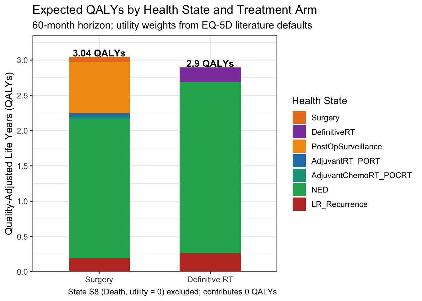
The intended users of the class of models I am proposing are physicians and their support teams who are making treatment decisions and explaining the possible consequences of the treatments to their patients. In the first use case, physicians may find the formality of the model and its baseline estimates useful in finalizing their decisions and documenting their decision making process. Having a model to inform treatment decisions should be especially helpful in situations where multiple physicians collaborate on deciding treatment options. At the very least, a model would be useful in verifying shared assumptions.
The second use of the model to help physicians and their care teams communicate with patients about the consequences of various treatment options is more speculative. To be truly helpful to patients physicians and their care teams must generate a compelling narrative for each health state explaining the side effects of the treatments experienced in each health state along with the strategies that previous patients have employed to cope with them. At the very least the exercise of explaining a journey through various states and interpreting the QALY’s may be useful in structuring patient conversations and setting expectations.
Five-year background survival for the general US population at age 62, \(S^{(5)}_{62}\), is computed from the 2021 SSA Period Life Table as the product of annual survival probabilities across ages 62 to 66:
\[S^{(5)}_{62} = \prod_{x=62}^{66}(1 - q_x)\]
where \(q_x\) is the one-year death probability at exact age \(x\) (SSA notation). Using the 2021 table values for ages 62–66: \(q_x^{\text{male}}\) = 0.01648, 0.01762, 0.01876, 0.01991, 0.02110 and \(q_x^{\text{female}}\) = 0.01014, 0.01085, 0.01155, 0.01222, 0.01295, giving \(S^{(5)}_{62} = 0.910\) (male) and \(0.944\) (female). The sex-weighted background survival is:
\[\bar{S}^{(5)} = w_M \cdot S^{(5)}_M + w_F \cdot S^{(5)}_F = 0.70 \times 0.910 + 0.30 \times 0.944 = 0.920\]
where the 70:30 sex split is from SEER oral cavity incidence data. Absolute five-year OS is then obtained as:
\[\text{OS}_{\text{abs}} = r \times \bar{S}^{(5)} = 0.84 \times 0.920 = 0.773\]
where \(r = 0.84\) is the SEER five-year relative survival for localized oral cavity cancer (Siegel et al. 2024, CA Cancer J Clin, Figure 5). The code below details this calculation and provides a sensitivity check at age 65 (note: age-65 values are pending verification).
# US Social Security Administration period life tables (2021 release, used for 2019 SEER cohort).
# 5-year survival probabilities by sex at age 62 (closest to OSCC median diagnosis age).
# Computed as prod(1 - q_x) for x = 62:66 from Table 4c6 (2021 Trustees Report cycle).
# Source: Social Security Administration. Period Life Table, 2021 (2024 Trustees Report).
# https://www.ssa.gov/oact/STATS/table4c6.html
surv_male_62   <- 0.9096  # 5-yr background survival, males age 62;   SSA 2021 prod(1-qx), x=62:66
surv_female_62 <- 0.9436  # 5-yr background survival, females age 62; SSA 2021 prod(1-qx), x=62:66

# OSCC sex distribution: ~70% male, ~30% female (SEER, oral cavity)
prop_male <- 0.70
expected_survival_5yr <- prop_male * surv_male_62 + (1 - prop_male) * surv_female_62

# SEER 5-year relative survival for localized oral cavity (Siegel 2024, Fig. 5)
relative_survival_5yr <- 0.84

# Absolute OS = relative survival × expected (background) survival
absolute_os_5yr <- relative_survival_5yr * expected_survival_5yr

# Sensitivity: 5-yr background survival at age 65 (upper end of median diagnosis age range).
# Source: Social Security Administration. Period Life Table, 2021 (2024 Trustees Report).
# Computed as prod(1 - q_x) for x = 65:69. https://www.ssa.gov/oact/STATS/table4c6.html
surv_male_65   <- 0.8923  # 5-yr background survival, males age 65;   SSA 2021 prod(1-qx), x=65:69
surv_female_65 <- 0.9320  # 5-yr background survival, females age 65; SSA 2021 prod(1-qx), x=65:69
expected_surv_65 <- prop_male * surv_male_65 + (1 - prop_male) * surv_female_65
absolute_os_65   <- relative_survival_5yr * expected_surv_65

data.frame(
  Assumption              = c("Age 62 (lower bound)", "Age 65 (upper bound)"),
  Background_5yr_survival = round(c(expected_survival_5yr, expected_surv_65), 3),
  Absolute_5yr_OS         = round(c(absolute_os_5yr, absolute_os_65), 3)
)
Assumption Background_5yr_survival Absolute_5yr_OS
1 Age 62 (lower bound) 0.920 0.773
2 Age 65 (upper bound) 0.904 0.760# Age 62: background survival 0.920 × relative survival 0.84 = 0.773 (~77%).
# Age 65 sensitivity: background survival 0.904 × relative survival 0.84 = 0.760 (~76%).There is no doubt that models based on real patient data would be more convincing. To this end, I have structured the format of the generated synthetic data file so that it is suitable for fitting a continuous time Markov chain using the R package msm. I have verified that msm is able to fit the eight state sample model from the synthetic data. It is reasonable to expect that models of similar complexity could be fit from real patient data.
The references in this section are neither complete nor definitive. The literature is enormous. They have been selected to support the default values for the user inputs.
Bernier et al. (2004) “Postoperative Irradiation with or without Concomitant Chemotherapy for Locally Advanced Head and Neck Cancer”, N Engl J Med. 350:1945–1952. PMID: 15128894. Landmark EORTC 22931 RCT establishing concurrent chemoRT as standard of care for high-risk post-operative HNSCC. Supports jump_P[5,6] and the locoregional control rates in the POCRT arm (S5).
Blatt et al. (2022) “Tumor Recurrence and Follow-Up Intervals in Oral Squamous Cell Carcinoma”, J Clin Med. 11(23):7061. PMID: 36498636. PMC: PMC9740063. DOI: 10.3390/jcm11237061. University Medical Centre Mainz, n = 760 OSCC patients. Supports S3 NED declaration timing ~24 months (mean recurrence interval 24 ± 26 months; 50% of recurrences by 24 months) and S3 mean sojourn revision to 22 months.
Brands et al. (2019) “Time Patterns of Recurrence and Second Primary Tumors in a Large Cohort of Patients Treated for Oral Cavity Cancer”, Cancer Med. 8(12):5810–5819. DOI: 10.1002/cam4.2124. Retrospective cohort of 594 OSCC patients; the great majority of recurrences occur in the first 2 years; 5-year cumulative second-event risk ~30%. Supports S3 sojourn revision to 22 months and S6 NED calibration.
Contrera et al. (2022) “Outcomes for Recurrent Oral Cavity Squamous Cell Carcinoma”, Oral Oncol. 134:106127. PMID: 36155359. DOI: 10.1016/j.oraloncology.2022.106127. MD Anderson, n = 259 salvage surgeries (1997-2011); 5-year OS 44.2% for surgical candidates vs. 1.5% for nonsurgical therapy; 51% second recurrence at median 17 months. Provides contextual support for the salvage surgery framework; primary source for current values jump_P[7,6] = 0.43 and jump_P[7,8] = 0.57 is Lee et al. (2024).
Cooper et al. (2004) “Postoperative Concurrent Radiotherapy and Chemotherapy for High-Risk Squamous-Cell Carcinoma of the Head and Neck”, N Engl J Med. 350:1937–1944. PMID: 15084618. RTOG 9501 RCT; locoregional control ~60% at 5 years in the concurrent chemoRT arm. Supports S5 jump probabilities.
Correia et al. (2026) “Timely Matters: Predictors of Delay in Oral Cavity Cancer Patients Across the Care Continuum”. Laryngoscope Investig Otolaryngol. 11(2):e70363. DOI: 10.1002/lio2.70363. (Also available via eScholarship. n = 93 OCSCC patients. Median surgery-to-adjuvant RT interval 8.4 weeks (same institution) and 9.3 weeks (different facility). Supports S1 mean sojourn revision to 1.5 months.
Dayan et al. (2023) “Predictors of prolonged treatment time intervals in oral cavity cancer”, Oral Oncol. 106622. DOI: 10.1016/j.oraloncology.2023.106622. CHUM Montreal, n = 145 multimodal OCSCC patients. Median surgery-to-PORT interval 64 days = 2.1 months. Supports S1 mean sojourn revision.
Goodwin (2000) “Salvage Surgery for Patients with Recurrent Squamous Cell Carcinoma of the Upper Aerodigestive Tract: When Do the Ends Justify the Means?”, Laryngoscope. 110(suppl 93):1–18. Cited in v2 for salvage success rate 15–25%. Superseded in v3 by Lee et al. 2024 for jump_P[7,6]; retained for historical context.
Graboyes et al. (2017) “Adherence to National Comprehensive Cancer Network Guidelines for Time to Initiation of Postoperative Radiation Therapy for Patients with Head and Neck Cancer”, Cancer. 123(14):2651–2660. DOI: 10.1002/cncr.30651. NCDB analysis, n = 47,273 HNSCC patients; over 50% failed to initiate PORT within the NCCN-recommended 6 weeks. Supports real-world S1 mean sojourn estimate of 1.5 months.
Hosni et al. (2019) “Predictors of Early Recurrence Prior to Planned Postoperative Radiation Therapy for Oral Cavity Squamous Cell Carcinoma and Outcomes Following Salvage Intensified Radiation Therapy”, Int J Radiat Oncol Biol Phys. 103(2):363–373. PMID: 30244160. Princess Margaret Cancer Centre, n = 601 OSCC patients (2003–2015); 3-year OS ~71% (95% CI 67–75%) after adjuvant PORT. Supports S4 jump probabilities (jump_P[4, 6:8]).
Katsoulakis et al. (2018) “Long-term outcomes in oral cavity squamous cell carcinoma with adjuvant and salvage radiotherapy after surgery”, Laryngoscope. PMID: 29637571. DOI: 10.1002/lary.27191. Memorial Sloan Kettering / VA Tampa; Evangelia Katsoulakis (first author). Provides contextual reference for the adjuvant RT pathway; jump_P[2,6] is now sourced from Dana-Farber Group 2011 and Studer et al. 2007 above.
Lee et al. (2024) “Clinical Outcome of Salvage Surgery in Patients with Recurrent Oral Cavity Cancer: A Systematic Review and Meta-Analysis”, Head Neck. 46(11):2901–2909. PMID: 39243149. DOI: 10.1002/hed.27928. 14 retrospective cohort studies, n = 2,069; pooled 5-year OS after salvage surgery = 43.0%; late-relapse subgroup 63.8% vs. 30.0% for early relapse. Primary source for jump_P[7,6] = 0.43 (salvage success) and jump_P[7,8] = 0.57 (mortality); revised from 0.25/0.75 — previous values over-estimated post-recurrence mortality relative to this pooled estimate.
Liu et al. (2007) “Impact of Recurrence Interval on Survival of Oral Cavity Squamous Cell Carcinoma Patients after Local Relapse”, Otolaryngol Head Neck Surg. 136(1):112–118. PMID: 17210345. DOI: 10.1016/j.otohns.2006.07.002. n = 1,687 oral cancer patients; 5-year OS after local recurrence 31.56%; recurrence within 18 months predicted higher mortality. Supports S7 sojourn of 12.5 months.
Mehanna et al. (2016) “PET-CT Surveillance versus Neck Dissection in Advanced Head and Neck Cancer”, N Engl J Med. 374(15):1444–1454. PMID: 26958921. DOI: 10.1056/NEJMoa1514493. PET-NECK RCT, n = 564 patients; response imaging performed at 12 weeks post-chemoradiotherapy; established ≥12-week post-RT interval as standard for response assessment in HNSCC. Supports S2 mean sojourn of 3.0 months (RT course 1.5 mo + ≥12-week response assessment window).
Luryi et al. (2014) “Positive Surgical Margins in Early Stage Oral Cavity Cancer: An Analysis of 20,602 Cases”, Otolaryngol Head Neck Surg. 151(6):984–990. PMID: 25210849. Large NCDB analysis of surgical margin rates and downstream outcomes in early-stage oral cavity cancer; early-stage N0 patients with negative margins have materially lower recurrence rates than all-stage series. Supports S3 transition probability framework, jump_P[3,7] = 0.18, and S6 NED calibration to 120 months.
Nathan et al. (2025) “The Influence of Reconstruction following Hemiglossectomy on Perioperative Outcomes”, Int J Otorhinolaryngol Head Neck Surg. DOI: 10.18203/issn.2454-5929.ijohns20252980. NSQIP database study, n = 866 hemiglossectomy patients (2008–2022); consistent with ~1–2% 30-day mortality in modern series. Supports jump_P[1,8] = 0.015.
Ord, Kolokythas & Reynolds (2006) “Surgical Salvage for Local and Regional Recurrence in Oral Cancer”, J Oral Maxillofac Surg. 64(9):1409–1414. PMID: 16916677. DOI: 10.1016/j.joms.2006.05.026. Reports outcomes of surgical salvage in recurrent oral cancer; data on local and regional recurrence rates and survival after primary surgery. Supports jump_P[3,7] = 0.18 (LR recurrence 12–18% for Stage II) and S3 mean sojourn revision to 22 months.
Sher et al. (2011) “Treatment of Oral Cavity Squamous Cell Carcinoma with Adjuvant or Definitive Intensity-Modulated Radiation Therapy”, Int J Radiat Oncol Biol Phys. 2011. PMID: 21531515. Dana-Farber Cancer Institute; n = 42 OCSCC (30 adjuvant IMRT, 12 definitive IMRT); Stage I–IV (24% Stage II); 2-yr LRC for definitive IMRT = 64%, 2-yr OS = 63%. Corroborated by Studer G, Zwahlen RA, Graetz KW et al. (2007), “IMRT in oral cavity cancer”, Radiat Oncol. 2:16. PMID: 17430599. DOI: 10.1186/1748-717X-2-16. University Hospital Zurich; n = 58 OCC IMRT patients; T1 LC = 95%; T2–4 and recurred stages LC ~50–60% at 2 years; definitive IMRT LC = 43% (but cohort was 69% T3/4 or recurred). Primary reference pair for jump_P[2,6] = 0.65 — definitive RT arm locoregional control for T2N0M0 Stage II; value is consistent with the early-stage subgroup in both series.
Shetty et al. (2022) “Salvage Surgery in Recurrent Oral Squamous Cell Carcinoma”, Front Oral Health. PMC8831824. Review of salvage surgery outcomes; radiation-naive recurrent OCSCC after salvage surgery: 5-year OS 59%, recurrence-free survival 60%. Provides supporting context for the salvage surgery framework; current value jump_P[7,6] = 0.43 is sourced from Lee et al. (2024).
Siegel et al. (2024) “Cancer Statistics, 2024”, CA Cancer J Clin. 74(1):12–49. PMID: 38230766. DOI: 10.3322/caac.21820. Annual American Cancer Society SEER-based statistics report. Figure 5 reports 5-year relative survival for localized oral cavity cancer (SEER localised stage, encompassing Stage I–II) as approximately 84% (diagnoses 2013–2019, follow-up through 2020). Note: relative survival overstates absolute OS — adjusting for sex-weighted background mortality from the SSA 2021 Period Life Table at median age 62 (\(\\bar{S}^{(5)} = 0.920\)) yields an estimated absolute 5-yr OS of approximately 77% (\(0.84 \\times 0.920 = 0.773\)) for Stage II localised oral cavity. Used as the primary population-level calibration benchmark for the Surgery arm.
Szturz et al. (2017) “Weekly Low-Dose Versus Three-Weekly High-Dose Cisplatin for Concurrent Chemoradiation in Locoregionally Advanced Non-Nasopharyngeal Head and Neck Cancer: A Systematic Review and Meta-Analysis”, Oncologist. 22(9):1056–1066. PMID: 28533474.
Tam et al. (2017) “Estimating Survival After Salvage Surgery for Recurrent Oral Cavity Cancer”, JAMA Otolaryngol Head Neck Surg. 143(7):685–690. PMID: 28448645. Reports survival outcomes following salvage surgery for recurrent oral cavity SCC. Supports S7 transition structure.
Tassone et al. (2023) “Going Off Guidelines: An NCDB Analysis of Missed Adjuvant Therapy Among Surgically Treated Oral Cavity Cancer”, Otolaryngol Head Neck Surg. 169(3):632–641. PMID: 36939392. DOI: 10.1002/ohn.205. NCDB analysis, n = 53,503; establishes PORT vs. POCRT indications and allocation rates. Supports jump_P[1,4] = 0.25 and jump_P[1,5] = 0.15.
Temam et al. (2005) “Treatment of the N0 Neck during Salvage Surgery after Radiotherapy of Head and Neck Squamous Cell Carcinoma”, Head Neck. 27(8):653–658. Cited in v2 for salvage success rates. Superseded in v3 by Lee et al. 2024; retained for historical context.
de Almeida et al. (2014) “Preferences and Utilities for Health States after Treatment for Oropharyngeal Cancer: Transoral Robotic Surgery versus Definitive (Chemo)radiotherapy”, Head Neck. 36(4):529–539. Reports EQ-5D utility values across treatment modalities; informs utility weights for treatment and NED states.
Govers et al. (2016) “Quality of Life after Different Procedures for Regional Control in Oral Cancer Patients: Cross-Sectional Survey”, Clin Otolaryngol. 41(3):228–235. EQ-5D-3L measurement in oral cavity OSCC patients following different regional treatment approaches.
Meregaglia & Cairns (2017) “A Systematic Literature Review of Health State Utility Values in Head and Neck Cancer”, Health Qual Life Outcomes. 15(1):174. DOI: 10.1186/s12955-017-0748-z. PMID: 28865475. Systematic review of 28 studies and 346 health state utility values in HNC; recommends EQ-5D as the preferred instrument. Confirms that evidence for recurrent and metastatic HNC states is sparse: the only patient-reported EQ-5D for recurrence found in the review is a median of 0.70 (del Barco et al. 2016), from a palliative-intent recurrent/metastatic cohort — a different clinical context from S7 (locoregional recurrence with potential salvage intent) in this model. The S7 utility of 0.55 is a modeller’s assumption informed by this evidence gap, not a directly reported value from this review.
Noel et al. (2015) “Comparison of Health State Utility Measures in Patients With Head and Neck Cancer”, JAMA Otolaryngol Head Neck Surg. 141(8):696–703. Prospective, cross-sectional, and longitudinal study of 100 patients with squamous cell carcinoma of the upper aerodigestive tract. Mean EQ-5D-5L = 0.82 three months post-treatment with no evidence of recurrence. Primary source for NED (S6) utility value.
Ramaekers et al. (2011) “The Impact of Late Treatment-Toxicity on Generic Health-Related Quality of Life in Head and Neck Cancer Patients after Radiotherapy”, Oral Oncol. 47(8):768–774. DOI: 10.1016/j.oraloncology.2011.05.012. Multi-centre cross-sectional survey; EQ-5D measured in HNC patients at least 6 months post-RT (late-effects survivorship cohort, not active treatment). Reports xerostomia and dysphagia as independent predictors of reduced utility post-RT. Retained as contextual reference for late RT toxicity; not the primary source for S4 (PORT) utility — that cohort does not represent patients during active adjuvant radiotherapy.
Sprave et al. (2022) “Patient Reported Outcomes Based on EQ-5D-5L Questionnaires in Head and Neck Cancer Patients: A Real-World Study”, BMC Cancer 22:1236. DOI: 10.1186/s12885-022-10346-4. PMID: 36447175. Freiburg University; n = 366 H&N cancer patients undergoing modern RT; prospective real-world PRO study; mean EQ-5D-5L at end of RT = 0.830 (SD not reported for full cohort). Primary source for S2 (Definitive RT) and S4 (PORT) utility weights = 0.83. Corroborated by Sprave et al. (2020, n=49): mean EQ-5D at RT completion = 0.828.
Sprave et al. (2020) “Characterization of Health-Related Quality of Life Based on the EQ-5D-5L Questionnaire in Head-and-Neck Cancer Patients Undergoing Modern Radiotherapy”, Expert Rev Pharmacoecon Outcomes Res. 20(6):673–682. DOI: 10.1080/14737167.2020.1823220. PMID: 32912005. Freiburg University Medical Center; n = 49 H&N cancer patients (57% definitive, 41% adjuvant RT); mean EQ-5D-5L at RT completion = 0.828 (SD 0.16). Corroborates Sprave 2022; supports S4 utility revision. Note: no significant permanent HRQOL deterioration observed at 6-month follow-up.
Truong et al. / RTOG 0522 (2017) “Quality of Life and Performance Status from a Substudy Conducted Within a Prospective Phase 3 Randomized Trial of Concurrent Accelerated Radiation Plus Cisplatin With or Without Cetuximab for Locally Advanced Head and Neck Carcinoma: NRG Oncology RTOG 0522”, Int J Radiat Oncol Biol Phys. 97(4):687–699. PMC5303682. PMID: 27727066. DOI: 10.1016/j.ijrobp.2016.08.003. Prospective phase III RCT, n = 818 analyzable patients (oropharynx, hypopharynx, larynx; Stage III–IV); EQ-5D-3L collected at pretreatment, last 2 weeks of treatment, 3 months, and annually. Reported EQ-5D values: baseline ~0.79 (CIS 0.78, CET/CIS 0.80); at 3 months from treatment start ~0.775 (CIS 0.78, CET/CIS 0.77); at 1 year ~0.84. Note: the EQ-5D value for the ‘within last 2 weeks of treatment’ time point was collected but not reported in the paper — the authors identified omission of an acute FACT-HN assessment as a study limitation. The 3-month value (0.775) is used as the closest available proxy for active-treatment utility in S5 (POCRT). Secondary limitation: cohort is definitively treated oropharynx/larynx (not postoperative oral cavity POCRT); adopted as best available CRT utility source. Comparison with Sprave et al. (2022): the Sprave 2022 adjuvant CRT cohort (baseline HI = 0.849, stable to RT completion; CRT vs RT-alone not significantly different at RT completion, p = 0.624) would support a value of ~0.83 for S5. The RTOG 0522-derived value of 0.775 is retained as a conservative estimate reflecting the higher toxicity of POCRT (high-dose cisplatin, post-surgical) relative to the mixed Sprave 2022 cohort. A sensitivity analysis using 0.83 would reduce the Surgery vs. Def RT QALY difference by ~0.009 QALYs. Primary source for S5 (POCRT) utility = 0.775. Not the primary source for S2 (RT alone); see Sprave et al. (2022).