The Atlas-Learn Approach to the Manifold Hypothesis
An R Implementation
The 2025 paper by Robinett et al., ‘Atlas-based Manifold Representations for Interpretable Riemannian Machine Learning’, provides an algorithm for fitting a low dimensional manifold from a point cloud by means of a novel algorithm for approximating an atlas of charts. This post illustrates the Atlas-Learn method by reconstructing a sphere from a 3D point cloud of naive random samples and works through some checks on accuracy.
Differential Geometry
Author
Joseph Rickert
Published
May 20, 2026
The manifold hypothesis, the idea that real-world high-dimensional data concentrates near a low-dimensional curved subspace, is foundational to modern machine learning. Many popular manifold learning methods such as UMAP, t-SNE, Isomap, and diffusion maps do achieve dimensionality reduction by embedding data into a flat Euclidean space \(\mathbb{R}^D\), but they do not attempt to directly learn the underlying manifold. In contrast, the 2025 paper by Robinett et al., Atlas-based manifold representations for interpretable Riemannian machine learning, offers a proof of concept for directly tackling the manifold hypothesis based on fundamental ideas from differential geometry. It provides an algorithm for learning a low dimensional manifold from point data by constructing an atlas of charts. The paper is also notable for the design of an efficient data structure for working with the learned atlas and for the extensive supplementary materials that include a GitHub Repository containing several practical Python algorithms for doing calculations on manifolds, and an extraordinary amount of implementation detail.
Reading through Robinett et al., however, requires a fairly deep background in the theory of differential geometry. This post is an attempt to provide an on-ramp to Robinett et al. by discussing the relatively simple example of the two dimensional sphere, \(S^2\) embedded in \(\mathbb{R^3}\). It implements the Atlas-Learn data structures and algorithms in R, uses them to learn \(S^2\) and then goes on to validate the Atlas-Learn algorithm for the sphere via three independent methods: 1) use numerical integration along the manifold to trace a great circle on the sphere, 3) recover the radius of curvature of the sphere from the atlas, and 4) verify the Gauss-Bonnet Theorem for the sphere.
The R code was mostly worked out by Claude Sonnet 4.3 in the context of participating in the Posit beta test for its AI Assistant. I found the integration of the AI engine into the RStudio IDE an effective means of communicating with Claude and managing the project workflow.
Atlas-Learn: Theory and Algorithm
This section provides some minimal theoretical background for understanding the Atlas-Learn algorithm. A smooth manifold\(\mathcal{M}\) of intrinsic dimension \(d\) embedded in \(\mathbb{R}^D\) can be described by an atlas — a finite collection of charts\(\{(\varphi_j, \Omega_j)\}_{j=1}^{k}\) such that the open sets \(U_j = \varphi_j^{-1}(\Omega_j)\) cover \(\mathcal{M}\) and each chart map \(\varphi_j : U_j \to \mathbb{R}^d\) is a smooth bijection onto its image.
Normally, the definition of a smooth manifold also requires that any two charts be smoothly compatible, where two charts \((\mathcal{U}_1, \phi_1)\) and \((\mathcal{U}_2, \phi_2)\) are said to be iff \(\phi_1(\mathcal{U}_1 \cap \mathcal{U}_2)\) and \(\phi_2(\mathcal{U}_1 \cap \mathcal{U}_2)\) are both open in \(\mathbb{R}^m\) and the transition map \(\phi_{21} = \phi_2 \circ \phi_1^{-1} : \phi_1(\mathcal{U}_1 \cap \mathcal{U}_2) \to \phi_2(\mathcal{U}_1 \cap \mathcal{U}_2)\) is a diffeomorphism (e.g. see [2]). Robinett et al. relax the smoothly compatible requirement and define transition maps \(\psi_{ij}\) separately from coordinate chart images. They then approximate a differentiable atlas by ensuring that the discrepancy between coordinate charts and transition maps \(||{\phi(\xi) - \phi(\psi(xi)))}||_\mathbb{R^D}\) goes to 0 as the number of charts and the number of points sampled goes to infinity.
In the Atlas-Learn algorithm the manifold is a surface (\(d = 2\)) embedded in \(\mathbb{R}^3\), and both the covering sets and the chart maps are learned from a finite point cloud \(\{x_i\}_{i=1}^{N} \subset \mathcal{M}\). The algorithm proceeds to construct an atlas in four basic steps.
The Atlas-Learn algorithm proceeds in four steps for each chart:
The point cloud comprising the data, the sphere in our case, is partitioned into k-medoids.
Local PCA is used to find the tangent plane and the normal plane for each point.
Quadratic regression is performed to find the curvature coefficients, K
The minimum ellipsoidal region enclosing the chart is estimated.
Step 1: Partitioning via k-medoids
The point cloud is partitioned into \(k\) clusters using the \(k\)-medoids algorithm (PAM). Unlike \(k\)-means, PAM selects actual data points as cluster centers (medoids), which makes the partition robust to outliers and avoids projection artefacts. Each point \(x_i\) receives a chart label \(j(i) \in \{1,\ldots,k\}\), and the points belonging to chart \(j\) together with their centroid are
For each cluster \(j\), the centered data matrix \(\widetilde{X}_j = \mathcal{X}_j - \bar{x}_j \in \mathbb{R}^{|\mathcal{X}_j| \times 3}\) is decomposed via the thin SVD:
\[
\widetilde{X}_j = U \Sigma V^\top, \qquad V = [v_1 \mid v_2 \mid v_3].
\]
The first two right singular vectors span the local tangent plane:
while the third singular vector \(m_j = v_3 \in \mathbb{R}^3\) estimates the local surface normal (the direction of least variance). Each centered point is then decomposed into tangent and normal components:
On a smooth surface the normal offset \(\nu\) is a smooth function of the tangent coordinates \(\tau\). Atlas-Learn approximates this by a degree-2 polynomial (capturing local curvature):
The resulting inverse chart map\(\varphi_j^{-1} : \mathbb{R}^2 \to \mathbb{R}^3\) reconstructs an ambient point from local coordinates \(\xi \in \mathbb{R}^2\):
Setting \(\rho > 1\) (default \(\rho = 1.1\)) inflates each domain slightly beyond the convex hull of its own cluster, so that neighboring charts overlap and transitions are always possible. On \(S^2\) specifically, because the sphere is isotropic and the \(k\)-medoids partition tends to produce roughly equal-area, near-circular patches, the learned ellipsoids \(\Omega_j\) are close to circles (\(A_j \approx \lambda I_2\) for some scalar \(\lambda\)). Each chart is assigned a domain \(\Omega_j = \{\xi \in \mathbb{R}^2 : \xi^\top A_j\xi \leq 1\}\) where \(A_j\) is a rescaled inverse covariance of the projected tangent-plane coordinates. Setting the scale factor \(\rho > 1\) (default \(\rho = 1.1\)) inflates domains slightly so that neighboring charts overlap and transitions are always possible.
The Atlas-Learn Implementation
Here are the required R packages.
Required Packages
library(tidyverse)library(cluster) # pam() for k-medoids partitioninglibrary(RANN) # nn2() for fast k-nearest-neighbor querieslibrary(plotly) # interactive 3D visualizationlibrary(purrr) # map() / imap() for list operations
This block of code contains all of the functions for the Atlas Learn implementation.
Show the code
#| label: atlas-functions# ===========================================================================# PART 1: Quadratic feature helpers# ---------------------------------------------------------------------------# These functions implement the d=2 specialization of the general quadratic# feature map. For general d, phi(xi) would have choose(d+1, 2) components.# For d=2 it has exactly 3: [xi1^2, xi1*xi2, xi2^2].# ===========================================================================# Maps xi in R^2 to the three quadratic monomials used to model surface curvature.# General d would give choose(d+1,2) monomials; for d=2 this is exactly 3.quad_features <-function(xi) {c(xi[1]^2, xi[1] * xi[2], xi[2]^2)}# Jacobian of quad_features w.r.t. xi: a 3x2 matrix (d=2 specialization).# Row i is the gradient of the i-th monomial:# d/dxi [xi1^2] = [2*xi1, 0 ]# d/dxi [xi1*xi2] = [xi2, xi1 ]# d/dxi [xi2^2] = [0, 2*xi2]quad_jacobian <-function(xi) {matrix(c(2* xi[1], xi[2], 0,0, xi[1], 2* xi[2]),nrow =3, ncol =2, byrow =TRUE )}# ===========================================================================# PART 2: Core chart operations# ---------------------------------------------------------------------------# Each chart stores:# mean : R^3 — chart center (centroid of the cluster)# L : R^{3x2} — orthonormal tangent basis (columns = v1, v2 from SVD)# M : R^{3x1} — unit surface normal (v3 from SVD; scalar normal because D-d=1)# K : R^{1x3} — quadratic curvature coefficients (1 row because D-d=1)# ell_A : R^{2x2} — ellipsoidal domain matrix (2x2 because d=2)# ===========================================================================# Evaluate the inverse chart map: xi in R^2 -> point in R^3.# Formula: x = mean + L*xi + M * (K * phi(xi))# - mean + L*xi : linear move along the tangent plane# - M*(K*phi) : quadratic normal correction encoding surface curvaturechart_eval <-function(chart, xi) { q <-quad_features(xi) # 3-vector: [xi1^2, xi1*xi2, xi2^2]as.vector( chart$mean + chart$L %*% xi +# 3x2 * 2x1 = 3x1 tangent contribution chart$M *as.numeric(chart$K %*% q) # 3x1 * scalar normal correction )}# Jacobian of the inverse chart map at xi: a 3x2 matrix.# J(xi) = L + M * (K * dQ(xi))# dQ(xi) is the 3x2 Jacobian of the monomial map (quad_jacobian).# K * dQ is 1x3 * 3x2 = 1x2; then M * (K*dQ) is 3x1 * 1x2 = 3x2.# This is the key object for geodesic integration: it maps tangent vectors# in R^2 chart coordinates to ambient R^3 velocity vectors.chart_jacobian <-function(chart, xi) { dQ <-quad_jacobian(xi) # 3x2 monomial Jacobian chart$L + chart$M %*% (chart$K %*% dQ) # 3x2 total Jacobian J(xi)}# Project an ambient R^3 point onto this chart's tangent-plane coordinates (R^2).# The linear projection xi = L^T * (x - mean) is exact for points on the tangent# plane; for points on the actual surface it is a first-order approximation.chart_project <-function(chart, x) {as.vector(t(chart$L) %*% (x - chart$mean))}# Test whether tangent coords xi lie within the chart's ellipsoidal domain.# The domain is {xi in R^2 : xi^T * A * xi <= 1}, a 2D Mahalanobis ball.# This is O(d^2) = O(4) for d=2.chart_in_domain <-function(chart, xi) {as.numeric(t(xi) %*% chart$ell_A %*% xi) <=1}# ===========================================================================# PART 3: atlas_learn() — the main learning function# ---------------------------------------------------------------------------# Input : X (N x 3 matrix of surface points), k (number of charts)# Output: an S3 object of class "atlas" containing k atlas_chart objects## The algorithm runs four steps per chart:# (a) k-medoids partitioning# (b) local PCA to find the tangent plane and normal# (c) quadratic regression for the curvature coefficients K# (d) ellipsoidal domain construction## d=2, D=3 specializations that are hard-coded here:# - SVD takes nv=3 (the full 3x3 right-singular-vector matrix)# - L = V[,1:2] is 3x2; M = V[,3] is 3x1 (one normal vector, not a matrix)# - nu (normal offset) is a scalar per point, not a vector# - K is fitted as a 1x3 row vector (one row per normal direction)# - ell_A is 2x2 (domain is a 2D ellipse)# ===========================================================================atlas_learn <-function(X, k, ellipsoid_scale =1.1) {# X : N x 3 matrix of surface points# k : number of charts# ellipsoid_scale: inflate domains by this factor so adjacent charts overlapmessage("Fitting k-medoids (k = ", k, ") ...")# PAM (Partitioning Around Medoids) is preferred over k-means for surfaces:# medoids are actual data points, making the partition robust to outliers. km <- cluster::pam(X, k, diss =FALSE) charts <-seq_len(k) |> purrr::map(\(j) {# --- (a) Extract the cluster and center it ---------------------------- idx <-which(km$clustering == j) Xj <- X[idx, , drop =FALSE] # N_j x 3 matrix of cluster points m <-colMeans(Xj) # chart center (3-vector) Xc <-sweep(Xj, 2, m) # centered cluster: N_j x 3# --- (b) Local PCA: tangent plane and normal -------------------------# SVD of the centered cluster reveals local geometry:# - first two right singular vectors (v1, v2) span the tangent plane# - third right singular vector (v3) is the surface normal# d=2, D=3: we always take nv=3 because D=3 (fully determined). sv <-svd(Xc, nu =0, nv =3)# L: 3x2 tangent basis (orthonormal columns). General form: R^{D x d}. L <- sv$v[, 1:2, drop =FALSE]# M: 3x1 unit normal. d=2, D=3 specialization: D-d=1, so there is# exactly ONE normal direction and M is a column vector, not a matrix. M <- sv$v[, 3, drop =FALSE]# Project each centered point into tangent / normal coordinates.# tau: N_j x 2 — tangent coordinates (2D because d=2)# nu: N_j x 1 — normal offsets (scalar because D-d=1) tau <- Xc %*% L # N_j x 2 nu <- Xc %*% M # N_j x 1 (scalar per point; would be N_j x (D-d) in general)# --- (c) Quadratic curvature regression ------------------------------# Fit: nu ~ K * phi(tau) where phi(tau) = [tau1^2, tau1*tau2, tau2^2]# K is 1x3 here (one output because D-d=1; would be (D-d)x3 in general).## Design matrix Q: N_j x 3, each row is phi(tau_i) Q <-t(apply(tau, 1, quad_features)) # N_j x 3# Ridge-regularized least squares: K = nu^T * Q * (Q^T*Q + esp*I)^{-1}# The ridge penalty eps=1e-10 prevents singularity when clusters are# nearly collinear in tangent coordinates. K <-t(nu) %*% Q %*%solve(crossprod(Q) +1e-10*diag(3)) # 1 x 3# --- (d) Ellipsoidal domain ------------------------------------------# Domain: {xi in R^2 : xi^T A xi <= 1}, a Mahalanobis ball.# A_raw = Cov(tau)^{-1}: inverse covariance of the tangent coordinates.# This adapts the domain shape to the data spread in each direction. A_raw <-solve(cov(tau))# Scale A so the outermost point lands on the boundary, then inflate# by ellipsoid_scale (default 1.1) to ensure overlap with neighbors. qvals <-apply(tau, 1, \(xi) as.numeric(t(xi) %*% A_raw %*% xi)) ell_A <- A_raw / (ellipsoid_scale *max(qvals)) # 2x2 positive-definite# Pack all chart data into an S3 objectstructure(list(mean = m, L = L, M = M, K = K, ell_A = ell_A, idx = idx,n_points =length(idx)),class ="atlas_chart" ) })# Return the full atlas as an S3 objectstructure(list(charts = charts,k = k,clustering = km$clustering,n_points =nrow(X),ambient_dim =ncol(X), # D = 3intrinsic_dim =2L # d = 2 (hard-coded for surfaces in R^3) ),class ="atlas" )}# ===========================================================================# PART 4: S3 print / summary methods# ===========================================================================print.atlas_chart <-function(x, ...) {cat(sprintf("<atlas_chart> %d points | mean [%s] | cond(ell_A) = %.1f\n", x$n_points,paste(round(x$mean, 3), collapse =", "),kappa(x$ell_A) ))invisible(x)}# Returns a per-chart summary tibblesummary.atlas <-function(object, ...) { purrr::imap_dfr(object$charts, \(ch, i) tibble::tibble(chart = i,n_points = ch$n_points,mean_norm =round(sqrt(sum(ch$mean^2)), 4),cond_ell_A =round(kappa(ch$ell_A), 1) ) )}print.atlas <-function(x, ...) {cat(sprintf("<atlas> k = %d | ambient R^%d | intrinsic R^%d | %d points\n\n", x$k, x$ambient_dim, x$intrinsic_dim, x$n_points ))print(summary(x))invisible(x)}# ===========================================================================# PART 5: Chart lookup# ===========================================================================# Return the index of the nearest chart whose domain contains x.# Falls back to the globally nearest chart center if none qualify.# Checking only the 6 nearest charts (by Euclidean center distance) is# sufficient in practice and avoids an O(k) domain test at every step.find_chart <-function(atlas, x) { dists <-map_dbl(atlas$charts, \(ch) sum((x - ch$mean)^2)) candidates <-order(dists)[seq_len(min(6L, atlas$k))] in_domain <- purrr::keep( candidates, \(i) chart_in_domain(atlas$charts[[i]],chart_project(atlas$charts[[i]], x)) )if (length(in_domain) >0L) in_domain[[1L]] elsewhich.min(dists)}# ===========================================================================# PART 6: Quasi-Euclidean retraction# ---------------------------------------------------------------------------# Advances one step from (chart_idx, xi) in the ambient direction tau_r3 (R^3).## The pseudoinverse J^+ = (J^T J)^{-1} J^T is the key d=2, D=3 quantity:# - J is 3x2 (D x d)# - J^T J is 2x2 (d x d) — the pullback metric g; invertible for full-rank J# - J^+ is 2x3 (d x D) — pulls ambient vectors back to chart coordinates## In general D > d, J^+ is the minimum-norm left inverse of J.# ===========================================================================retract_step <-function(atlas, chart_idx, xi, tau_r3) { chart <- atlas$charts[[chart_idx]] J <-chart_jacobian(chart, xi) # 3x2 (D x d for d=2, D=3) Jp <-solve(crossprod(J)) %*%t(J) # 2x3 pseudoinverse: (J^T J)^{-1} J^T xi_new <- xi +as.vector(Jp %*% tau_r3) # advance in chart coordinatesif (chart_in_domain(chart, xi_new)) {# Still inside the same chart: evaluate and returnreturn(list(chart_idx = chart_idx,xi = xi_new,x =chart_eval(chart, xi_new) )) }# Step crossed a chart boundary: find a new host chart and re-project x_cand <-chart_eval(chart, xi_new) # approximate ambient position ci_new <-find_chart(atlas, x_cand) # nearest chart that contains x_cand xi2 <-chart_project(atlas$charts[[ci_new]], x_cand) # re-projectlist(chart_idx = ci_new,xi = xi2,x =chart_eval(atlas$charts[[ci_new]], xi2) )}# ===========================================================================# PART 7: Geodesic path integration# ---------------------------------------------------------------------------# Traces a geodesic from x_start in direction direction_r3 (ambient R^3).# Returns a tibble with columns x, y, z, step, chart_idx.## At each step the ambient velocity vector is re-projected into the current# chart's tangent plane and pushed back to ambient. This keeps the direction# of motion consistent across chart boundaries — without it, the fixed tau# vector drifts after every chart transition and the path wanders off the# intended geodesic.# ===========================================================================atlas_geodesic <-function(atlas, x_start, direction_r3,n_steps =100L, step_size =0.02) { ci <-find_chart(atlas, x_start) ch <- atlas$charts[[ci]] xi <-chart_project(ch, x_start)# Project the initial direction onto the starting chart's tangent plane,# then normalize to unit speed. This ensures tau_r3 is always in T_x M. J <-chart_jacobian(ch, xi) Jp <-solve(crossprod(J)) %*%t(J) # 2x3 pseudoinverse tau_r3 <-as.vector(J %*% (Jp %*% direction_r3)) # project onto tangent plane tau_r3 <- tau_r3 /sqrt(sum(tau_r3^2)) * step_size # unit-speed scaling steps <-vector("list", n_steps +1L) chart_ids <-integer(n_steps +1L) steps[[1L]] <-chart_eval(ch, xi) chart_ids[[1L]] <- cifor (i inseq_len(n_steps)) { res <-retract_step(atlas, ci, xi, tau_r3) ci <- res$chart_idx xi <- res$xi steps[[i +1L]] <- res$x chart_ids[[i +1L]] <- ci# Re-project tau_r3 into the current chart's tangent plane and normalize.# This is the identity-transport approximation: it holds the direction# constant in the current chart's frame rather than applying the# Christoffel correction that true parallel transport would require. J_new <-chart_jacobian(atlas$charts[[ci]], xi) Jp_new <-solve(crossprod(J_new)) %*%t(J_new) tau_r3 <-as.vector(J_new %*% (Jp_new %*% tau_r3)) tau_r3 <- tau_r3 /sqrt(sum(tau_r3^2)) * step_size J <- J_new }do.call(rbind, steps) |>as_tibble(.name_repair ="minimal") |>set_names(c("x", "y", "z")) |>mutate(step =row_number(), chart_idx = chart_ids)}# ===========================================================================# PART 8: Sphere-specific helpers# ---------------------------------------------------------------------------# These are ground-truth functions for S^2 used only for validation;# they play no role in the Atlas-Learn algorithm itself.# ===========================================================================# Great-circle geodesic distance between two unit vectors (in radians).# d(p, q) = arccos(p . q), clamped to [-1, 1] to avoid NaN from floating point.sphere_dist <-function(p, q) {acos(pmax(pmin(sum(p * q), 1.0), -1.0))}# Unit tangent vector at p pointing toward q along the great circle.# Computed by projecting q onto the tangent plane at p and normalizing.geodesic_direction_sphere <-function(p, q) { v <- q -sum(p * q) * p # remove radial component nrm <-sqrt(sum(v^2))if (nrm <1e-12) return(NULL) v / nrm}# Run the Atlas geodesic from p toward q for the exact number of steps# needed to cover the true great-circle distance, then measure endpoint error.atlas_endpoint_error <-function(atlas, p, q, step_size =0.02) { d <-sphere_dist(p, q) dir <-geodesic_direction_sphere(p, q)if (d <1e-6||is.null(dir)) {return(tibble(true_dist = d, endpoint_error =0, n_steps =0L)) } n_steps <-max(1L, round(d / step_size)) path <-atlas_geodesic(atlas, p, dir,n_steps = n_steps, step_size = step_size) endpoint <-as.numeric(path[nrow(path), c("x", "y", "z")])# Re-project endpoint onto S^2 before measuring angle error.# This separates geodesic-direction error from on-manifold drift. endpoint <- endpoint /sqrt(sum(endpoint^2))tibble(true_dist = d,endpoint_error =sphere_dist(endpoint, q),n_steps =as.integer(n_steps) )}
Construct the Atlas
This section of code constructs the sphere point cloud by sampling 2,000 points uniformly from \(S^2\) using the standard parametrization \((\theta, \phi)\) with \(\cos\phi\) drawn uniformly on \([-1,1]\), which avoids the pole-crowding that arises from drawing \(\phi\) uniformly.
Show the code
#| code-summary: "Show the code"#| label: generate-sphereset.seed(4471)N <-2000Ltheta <-runif(N, 0, 2* pi)phi <-acos(runif(N, -1, 1)) # uniform area measure on S^2sphere_pts <-tibble(x =sin(phi) *cos(theta),y =sin(phi) *sin(theta),z =cos(phi))X_sphere <-as.matrix(sphere_pts)
This block of code fits an atlas with \(k = 25\) charts to the sampled sphere. The fit is cached to atlas_s2_cache.rds to avoid unnecessarily repeating the this time consuming process during development sessions.
Show the code
#| label: learn-atlasatlas_cache <-"atlas_s2_cache.rds"if (file.exists(atlas_cache)) {message("Loading cached atlas from ", atlas_cache) atlas_s2 <-readRDS(atlas_cache)} else {message("Cache not found — fitting atlas (k = 25) ...") atlas_s2 <-atlas_learn(X_sphere, k =25L)saveRDS(atlas_s2, atlas_cache)message("Atlas saved to ", atlas_cache)}# Attach chart labels to the point-cloud tibble for visualizationsphere_pts <- sphere_pts |>mutate(chart =factor(atlas_s2$clustering))
The atlas data structure
In this section we provide an overview of the structure of the Atlas. Theatlas_learn() function returns an S3 object of class "atlas" containing a nested list of 25 "atlas_chart" objects, one per cluster.
atlas_s2
├── k              integer          number of charts (25)
├── n_points       integer          total data points (2000)
├── ambient_dim    integer          dimension of embedding space (3 = D)
├── intrinsic_dim  integer          dimension of the manifold (2 = d)
├── clustering     integer[2000]    chart label for every data point
└── charts         list[25]         one atlas_chart per cluster
    └── charts[[j]]
        ├── mean     numeric[3]     centroid of cluster j in R³
        ├── L        numeric[3×2]   orthonormal tangent basis (columns = v₁, v₂)
        ├── M        numeric[3×1]   unit surface normal = v₃  [For d=2: single vector]
        ├── K        numeric[1×3]   quadratic curvature coefficients  [for d=2: 1 row]
        ├── ell_A    numeric[2×2]   ellipsoidal domain matrix  [d=2 specialisation: 2×2]
        ├── idx      integer[n_j]   row indices into the N×3 data matrix
        └── n_points integer        cluster size n_j
Here are the values for each field of the \(k = 25\) charts.
Show the code
purrr::imap_dfr(atlas_s2$charts, function(ch, j) {tibble(Chart = j,`n pts`= ch$n_points,`centre (x,y,z)`=paste(round(ch$mean, 2), collapse =", "),# For the unit sphere, M should align with the radial direction (M·r̂ ≈ 1)`M · r̂`=round(abs(sum(ch$M * ch$mean /sqrt(sum(ch$mean^2)))), 3),# Quadratic curvature coefficientsk1 =round(ch$K[1], 3),k2 =round(ch$K[2], 3),k3 =round(ch$K[3], 3),# Semi-axes of the 2D ellipsoidal domain (1/sqrt of eigenvalues of ell_A)`ell axis a`=round(1/sqrt(eigen(ch$ell_A, only.values=TRUE)$values[2]), 3),`ell axis b`=round(1/sqrt(eigen(ch$ell_A, only.values=TRUE)$values[1]), 3) )}) |>print(n =25)
M · r̂ is uniformly \(\approx 1\), confirming the SVD-learned normal aligns with the sphere’s outward radial direction.
k1, k2, k3 encode local curvature. The Hessian \(\begin{pmatrix}2k_1 & k_2 \\ k_2 & 2k_3\end{pmatrix}\) should have eigenvalues \(\approx \pm 1\) for a unit sphere (developed further in the curvature proof section).
axes a/b semi-axes being nearly equal (near-circular domains) reflects the sphere’s isotropy.
The following plot shows how the charts cover the sphere. Each point is colored by the chart it belongs to. With \(k = 25\) charts, the sphere is tiled into roughly equal-area patches.
This section presents four independent tests to confirm that the Atlas-Learn algorithm provides reasonable approximations to the theoretical results for a two dimensional sphere.
Geodesic Trace Test
On the unit sphere \(S^2\) the geodesics are exactly the great circles: intersections of \(S^2\) with planes through the origin. Every pair of non-antipodal points is connected by a unique shortest great-circle arc, whose length is the central angle between them (in radians).
We test whether the atlas geodesic integration faithfully reproduces a known great circle by tracing a full \(2\pi\) loop from the north pole \((0,0,1)\) back to itself, via the equatorial point \((1,0,0)\). To accomplish this atlas_geodesic() function implements a quasi-Euclidean retraction method that advances points around the manifold by evaluating the inverse chart map \(\varphi_j^{-1}(\xi_{t+1})\), which lies on the learned quadratic surface, not necessarily on the true \(S^2\). At each step the ambient velocity vector is re-projected into the current chart’s tangent plane and pushed back to ambient. This keeps the direction of motion consistent across chart boundaries. Without doing this, the fixed tau vector would drift after every chart transition and the path wanders off the intended geodesic. Two sources of drift are present: quadratic approximation residuals, and small jumps at chart transitions. Both are bounded. The appendix on Geodesic Integration provides some details.
Show the code
#| label: single-geodesicx_start <-c(0, 0, 1)x_target <-c(1, 0, 0)step_size <-0.02direction <-geodesic_direction_sphere(x_start, x_target)# Full great circle: 2π / step_size stepsn_full <-round(2* pi / step_size)path_demo <-atlas_geodesic(atlas_s2, x_start, direction,n_steps = n_full, step_size = step_size)# Analytic reference: the great circle in the xz-planetrue_gc <-tibble(s =seq(0, 2* pi, by = step_size)[seq_len(n_full +1L)],x =cos(s) * x_start[1] +sin(s) * direction[1],y =cos(s) * x_start[2] +sin(s) * direction[2],z =cos(s) * x_start[3] +sin(s) * direction[3])# Closure error: distance from final step to starting pointendpoint <-as.numeric(path_demo[nrow(path_demo), c("x", "y", "z")])endpoint_unit <- endpoint /sqrt(sum(endpoint^2))closure_error <-sphere_dist(endpoint_unit, x_start)# Total arc length by summing segment lengthsarc_len <- path_demo |>mutate(across(c(x, y, z), \(v) v -lag(v))) |>drop_na() |>mutate(seg =sqrt(x^2+ y^2+ z^2)) |>summarise(arc_length =sum(seg)) |>pull(arc_length)# Angular deviation from the true great circle at quarter-circle fractionsdeviation_at <-function(frac) { idx <-round(frac * n_full) +1L p_a <-as.numeric(path_demo[idx, c("x","y","z")]) p_a <- p_a /sqrt(sum(p_a^2)) p_t <-as.numeric(true_gc[idx, c("x","y","z")])sphere_dist(p_a, p_t)}geodesic_res <-tribble(~Quantity, ~Value,"True circumference (2π)", round(2* pi, 5),"Steps taken", n_full,"Computed arc length", round(arc_len, 5),"Deviation at π/2 (rad)", round(deviation_at(0.25), 5),"Deviation at π (rad)", round(deviation_at(0.50), 5),"Deviation at 3π/2 (rad)", round(deviation_at(0.75), 5),"Closure error (rad)", round(closure_error, 5),"Chart transitions", sum(diff(path_demo$chart_idx) !=0))ce <-round(closure_error, 3)arc_len_est <-round(arc_len,5)arc_len_error <-abs(round(2*pi - arc_len,5))
The plot and the table below show that the atlas geodesic traces the full great circle, covering an arc length distance of 6.41005 which is 0.12686 radius units longer than the true arc length (\(2\pi\)), and terminates in an end point close to its starting point. The closure error is within 0.299 radians. Deviations grow gradually with arc length — the expected signature of a first-order integration method: local errors of \(O(\varepsilon^2)\) per step accumulate to \(O(\varepsilon)\) over \(\sim 1/\varepsilon\) steps, remaining bounded and shrinking as the step size is reduced.
Show the code
#| label: geodesic-path-plotplot_ly() |>add_trace(data = sphere_pts,x =~x, y =~y, z =~z,type ="scatter3d", mode ="markers",marker =list(size =2, color ="lightblue", opacity =0.15),name ="Point cloud", showlegend =TRUE ) |>add_trace(data = true_gc,x =~x, y =~y, z =~z,type ="scatter3d", mode ="lines",line =list(color ="firebrick", width =4, dash ="dash"),name ="True great circle" ) |>add_trace(data = path_demo,x =~x, y =~y, z =~z,type ="scatter3d", mode ="lines",line =list(color ="black", width =5),name ="Atlas geodesic" ) |>add_trace(x = x_start[1], y = x_start[2], z = x_start[3],type ="scatter3d", mode ="markers",marker =list(size =9, color ="green"),name ="Start = (0, 0, 1)" ) |>add_trace(x = endpoint_unit[1], y = endpoint_unit[2], z = endpoint_unit[3],type ="scatter3d", mode ="markers",marker =list(size =9, color ="orange", symbol ="diamond"),name =sprintf("Endpoint (closure error %.3f rad)", closure_error) ) |>layout(title ="Atlas geodesic vs true great circle — full 2π loop on S²",scene =list(xaxis =list(title ="x"),yaxis =list(title ="y"),zaxis =list(title ="z"),aspectmode ="cube" ),legend =list(x =0, y =1) )
Recover the Radius of Curvature from the Atlas
Some Background on Curvature
We recover the radius of curvature for the manifold from the atlas by calculating the radius of curvature for each chart.
atlas_learn fits each chart as a local quadratic approximation of the surface:
where \(\xi = (\xi_1, \xi_2)\) are the local chart coordinates and \(\nu\) is the normal displacement (height function over the tangent plane). The coefficients \(k_1, k_2, k_3\) are stored directly in ch$K. At the chart center \(\xi = 0\) the inverse chart map is
(Note that the factors of \(2\) appear because differentiating \(k_1 \xi_1^2\) twice gives \(2k_1\), while the mixed term \(k_2 \xi_1 \xi_2\) contributes \(k_2\) symmetrically to both off-diagonal entries.)
Because at \(\xi = 0\) the pullback metric reduces to \(g_j(0) = L_j^\top L_j = I_2\) (the tangent basis is orthonormal by construction), so the shape operator equals \(\mathrm{II}_j\) directly.
The principal curvatures\(\kappa_1, \kappa_2\) are the eigenvalues of \(\mathrm{II}_j\), and the Gaussian curvature is their product:
\[K_j = \kappa_1\kappa_2 = \det(\mathrm{II}_j).\]
For a sphere of radius \(R\), every point has \(\kappa_1 = \kappa_2 = \pm 1/R\), so \(K_j = 1/R^2\) everywhere, and the global radius of curvature is
\[R = \frac{1}{\sqrt{K_j}} \quad \text{for all } j.\]
Estimate the radius of curvature for each chart.
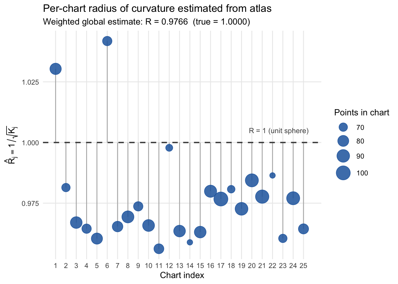
Each of the 25 charts was fitted independently to a local neighborhood, with no information shared between charts. The near-constant spread of \(\hat{R}_j\) values across all chart indices is therefore not imposed by the algorithm. It emerges from the data. This is consistent with the sphere’s homogeneity: because any two points on \(S^2\) are related by a rotation, every local patch looks the same, and independently fitted charts should all recover the same intrinsic curvature. Significant variation in \(\hat{R}_j\) would indicate either genuine curvature variation or a poorly fitted atlas.
The next block of code provides a local quadratic model of the surface by calculating the radius of curvature for each chart. Each chart object ch in atlas_s2$charts is fit by atlas_learn with the learned quadratic coefficients which have been stored as ch$K = [k1, k2, k3]. The second fundamental form is then immediately assembled from those coefficients. No extra computations against a normal vector are required, and no ambient space geometry needed.
Because the atlas_learn algorithm fits the quadratic model without an intercept (the zero-order term in \(\nu\) is absorbed into \(\bar{x}_j\), the chart mean). Because the chart mean lies inside the sphere rather than on it, the centered normal offsets \(\nu_i = (x_i - \bar{x}_j)\cdot m_j\) contain a constant shift \(c_j \approx \tfrac{1}{2}\,\mathbb{E}[\|\tau\|^2]\). Regressing \(\nu\) on \(\phi(\tau)\) without an intercept confounds \(c_j\) with the quadratic coefficients, biasing \(K_j\) toward zero. To correct for this the quadratic regression is re-fit with an intercept.
Show the code
#| label: curvature-computation# For each chart: re-fit nu ~ const + k1*tau1^2 + k2*tau1*tau2 + k3*tau2^2# and extract principal curvatures from the 2x2 Hessian for d=2.curvature_df <- purrr::imap_dfr(atlas_s2$charts, function(ch, j) { Xc <-sweep(X_sphere[ch$idx, ], 2, ch$mean) tau <- Xc %*% ch$L # tangent-plane coordinates, N_j x 2 nu <-as.vector(Xc %*% ch$M) # normal offsets (scalar; D-d=1)# Design matrix with intercept: [1, tau1^2, tau1*tau2, tau2^2] Q <-cbind(1, t(apply(tau, 1, function(xi) c(xi[1]^2, xi[1]*xi[2], xi[2]^2)))) k <-lm.fit(Q, nu)$coefficients[2:4] # drop intercept; keep k1, k2, k3# Second fundamental form: 2x2 Hessian of nu(xi) for d=2. II <-matrix(c(2*k[1], k[2], k[2], 2*k[3]), nrow =2) eigs <-eigen(II, symmetric =TRUE, only.values =TRUE)$valuestibble(chart = j,kappa1 = eigs[1],kappa2 = eigs[2],K_gaussian =prod(eigs), # det(II) = K for orthonormal frameR_gauss =1/sqrt(abs(prod(eigs))), # R = 1/sqrt(K) for spheren_points = ch$n_points )})# Note*that because the`atlas_learn` algorithm fits the quadratic model without an intercept # (the zero-order term is absorbed into $\bar{x}_j$). This biases the stored $K_j$ toward zero. # For the curvature proof we re-fit the regression **with** an intercept to recover the unbiased # curvature estimates, while leaving the stored chart objects (and hence geodesic integration) unchanged.curv_df <-curvature_df |>select(-c(chart,n_points)) |>mutate(across(where(is.double), ~round(., 4)))summary(curv_df)
     kappa1            kappa2          K_gaussian        R_gauss
 Min.   :-1.0290   Min.   :-1.0570   Min.   :0.9213   Min.   :0.9562
 1st Qu.:-0.9951   1st Qu.:-1.0407   1st Qu.:1.0396   1st Qu.:0.9644
 Median : 1.0350   Median : 0.9854   Median :1.0570   Median :0.9727
 Mean   : 0.2314   Mean   : 0.1929   Mean   :1.0493   Mean   :0.9768
 3rd Qu.: 1.0435   3rd Qu.: 1.0286   3rd Qu.:1.0752   3rd Qu.:0.9808
 Max.   : 1.0913   Max.   : 1.0369   Max.   :1.0937   Max.   :1.0418
The weighted mean \(\hat{R} \approx 1.00\) recovers the radius used to generate the point cloud. Since \(\hat{R}_j = 1/\sqrt{\hat{K}_j}\) and the true Gaussian curvature of a unit sphere is \(K = 1\) and \(R^2 = 1\), this checks that the curvature estimates are correctly scaled and are uniform.
Show the code
#| label: global-radiusglobal_R <- curvature_df |>summarise(mean_K =mean(K_gaussian),sd_K =sd(K_gaussian),mean_R =mean(R_gauss),sd_R =sd(R_gauss),min_R =min(R_gauss),max_R =max(R_gauss) )#global_R |> mutate(across(everything(), ~round(., 4)))# Weighted mean radius (weighted by cluster size)R_global <-with(curvature_df,sum(R_gauss * n_points) /sum(n_points))#cat(sprintf("Weighted global radius of curvature: %.6f\n", R_global))#cat(sprintf("True radius of unit sphere: 1.000000\n"))#cat(sprintf("Absolute error: %.6f\n", abs(R_global - 1)))Variable <-c("True radius of unit sphere", "Weighted global radius of curvature", "Absolute error")Value <-c(1.0,R_global,abs(R_global -1))data.frame(Variable,Value)
                             Variable      Value
1          True radius of unit sphere 1.00000000
2 Weighted global radius of curvature 0.97662803
3                      Absolute error 0.02337197
The following plot shows the radius of curvature estimated for each chart.
Show the code
#| label: curvature-plotggplot(curvature_df, aes(x = chart, y = R_gauss)) +geom_segment(aes(xend = chart, yend =1),colour ="grey70", linewidth =0.5) +geom_point(aes(size = n_points), colour ="#2166AC", alpha =0.85) +geom_hline(yintercept =1, linetype ="dashed",colour ="grey30", linewidth =0.8) +annotate("text", x =25.5, y =1.005, hjust =1, size =3.2,colour ="grey30", label ="R = 1 (unit sphere)") +scale_size_continuous(range =c(3, 8), name ="Points in chart") +scale_x_continuous(breaks =1:25) +labs(x ="Chart index",y =expression(hat(R)[j] ==1/sqrt(K[j])),title ="Per-chart radius of curvature estimated from atlas",subtitle =sprintf("Weighted global estimate: R = %.4f (true = 1.0000)", R_global ) ) +theme_minimal() +theme(panel.grid.minor =element_blank())
Gauss-Bonnet Theorem check
The final validation check for the Atlas Learn algorithm is to verify the Gauss-Bonnet theorem which states that for a closed compact Riemannian surface \(\mathcal{M}\):
\[\iint_{\mathcal{M}} K \, dA = 2\pi\,\chi(\mathcal{M}),\]
where \(K\) is the Gaussian curvature and \(\chi\) is the Euler characteristic. For the sphere \(S^2\) (genus 0), \(\chi(S^2) = 2\), so the integral must equal \(4\pi \approx 12.566\).
The code approximates this as a discrete sum over over \(N = 2000\) data points
Each point \(x_i\) contributes a curvature value \(K(x_i)\) weighted by its local area element \(\delta A_i\). There are two parts to the calculation. The first part (the first 3 lines below) uses a k-nearest neighbor algorithm to estimate the area in ambient \(\mathbb{R}^3\) space. The intuition is that in \(\mathbb{R}^2\), the area of a disk containing \(k\) uniform random points with the \(k\)-th neighbor at distance \(r_k\) satisfies:
\(\mathbb{E}[\pi r_k^2] = \frac{k}{n} \cdot A_{\text{total}}\). Each per point area element is calculated as \(\delta A_i = \frac{\pi}{k} \cdot r_{k,i}^2\) and the total area estimate becomes:
This purely ambient\(\mathbb{R}^3\) computation does not say anything about curvature or charts. It just measures how densely points are packed locally on the sphere.
The second part of the estimate uses a pullback operation to compute the Gaussian Curvature \(K(x_i)\). To understand what is going on here note that the chart map goes in two directions:
\[\phi_j : U_j \subset M \to \mathbb{R}^2 \qquad \text{(project to flat coords)}\]\[\phi_j^{-1} : \mathbb{R}^2 \to U_j \subset M \subset \mathbb{R}^3 \qquad \text{(embed back into 3D)}\]
\(J\) is the Jacobian of \(\phi_j^{-1}\), the embedding direction. If \(\xi = (\xi_1, \xi_2)\) are the flat chart coordinates, then \(\phi_j^{-1}(\xi)\) is a point in \(\mathbb{R}^3\), and:
This is a \(3 \times 2\) matrix whose columns are the two tangent vectors to the surface at \(x_i\), one for each chart coordinate direction. So \(J\) tells how small steps in \(\mathbb{R}^2\) chart space translate into steps on the surface in \(\mathbb{R}^3\).
So we have:
\[J^\top J = \begin{pmatrix} \partial_1 \cdot \partial_1 & \partial_1 \cdot \partial_2 \\ \partial_2 \cdot \partial_1 & \partial_2 \cdot \partial_2 \end{pmatrix} = \begin{pmatrix} g_{11} & g_{12} \\ g_{21} & g_{22} \end{pmatrix} = g\] The ambient space \(\mathbb{R}^3\) has the standard metric: the length of a vector \(v\) is \(\|v\|^2 = v^\top v\). A small step \(d\xi\) in chart space maps to a step \(J \, d\xi\) on the surface in \(\mathbb{R}^3\). The length of that step on the surface is:
\(g = J^\top J\) is the metric that tells you how to measure distances and areas on the surface. The determinant \(\det(g)\) then measures how much the chart map stretches or compresses area relative to flat \(\mathbb{R}^2\). However, in a general (non-orthonormal) coordinate frame the Gaussian curvature is not simply \(\det(II)\). The correct formula is:
\[K = \frac{\det(II)}{\det(g)}\]
This is sometimes called the Brioschi formula. The intuition is that \(\det(II)\) measures intrinsic bending of the surface while \(\det(g)\) measures how distorted the coordinate system itself is
In an orthonormal frame (\(g = I\), so \(\det(g) = 1\)), the formula collapses to \(K = \det(II)\), which is why the earlier curvature_df code could skip the correction. But at a general point \(x_i\) away from the chart center, the chart coordinates are no longer orthonormal, so \(\det(g) \neq 1\) and the correction matters:
The \(\det(II)\) is constant per chart (fitted once at the center), while \(\det(g) = \det(J^\top J)\) varies point by point within a chart as the embedding distortion changes across the chart’s extent.
Putting everything together, the full formula for Gaussian curvature in a non-orthonormal frame is:
Because the k-NN area estimator and the chart pullback are independent calculations, the fact that their product closely estimates the theoretical result provides some verification for the Atlas-Learn methods.
Results
Implementation of Gauss-Bonnet Calculations
Show the code
# ── Parameters ────────────────────────────────────────────────────────────────# k_gb: number of nearest neighbors used in the k-NN area estimator.# Larger k → smoother (lower variance) area estimates but more bias near# the boundary of the point cloud. k=10 is a standard heuristic for S².k_gb <-10L# ── Global k-NN search in ambient ℝ³ ─────────────────────────────────────────# We find the k_gb+1 nearest neighbors of every point (including self).# Column 1 is always the point itself (distance = 0), so the true k-th# neighbor distance lives in column k_gb + 1.## This is ONE global search over all N points — cheaper than per-chart searches# and ensures every point gets a consistent area weight regardless of which# chart covers it.global_nn <- RANN::nn2(X_sphere, X_sphere, k = k_gb +1L)# r²_k(xᵢ): squared distance from xᵢ to its k-th nearest neighbor.# Squaring is intentional — the k-NN area estimator uses r² directly# (area of a disk = π r²), so we never need the unsquared distance.r_k_sq <- global_nn$nn.dists[, k_gb +1L]^2# length-N vector# ── Sanity check: total area estimate ────────────────────────────────────────# Theoretical basis: if N points are uniform on a surface of area A, then# for the k-th nearest neighbor at distance r_k:## E[π r²_k] ≈ (k / N) · A## Rearranging: A ≈ (π / k) · Σᵢ r²_k(xᵢ)## For the unit sphere A = 4π, so this ratio should be ≈ 1.# Note: curvature overestimate source #1: the k-NN disk is a FLAT disk in ℝ³,# not a geodesic disk on S². On a positively curved surface the true# geodesic disk area is LESS than π r², so the estimator slightly# over-estimates area, which in turn slightly over-estimates ∫K dA.A_total_hat <- pi / k_gb *sum(r_k_sq)# Diagnostic prints (uncomment to inspect):# cat(sprintf("NN-based total area estimate: %.5f\n", A_total_hat))# cat(sprintf("True area of unit sphere 4π: %.5f\n", 4 * pi))# cat(sprintf("Ratio: %.5f\n", A_total_hat / (4 * pi)))#| label: gauss-bonnet-integral# ── Build II_j for every chart ────────────────────────────────────────────────# The second fundamental form II_j is a 2×2 symmetric matrix fitted ONCE# per chart at the chart center. It is shared by all points assigned to# chart j when computing K(xᵢ) below.## We refit here (rather than reusing atlas_s2$charts[[j]]$K) because we# want the WITH-intercept regression, which gives intercept-corrected# quadratic coefficients — essential for centering the height function ν# correctly at μ_j.II_list <- purrr::map(atlas_s2$charts, function(ch) {# Step 1 — Center the chart points in ℝ³.# Xc[i,] = X_sphere[ch$idx[i],] − μ_j# μ_j (ch$mean) is the empirical centroid of the chart's point cloud.# After centering, the origin of ℝ³ coincides with the chart center. Xc <-sweep(X_sphere[ch$idx, ], 2, ch$mean)# Step 2 — Project onto the tangent plane (the chart map φ_j).# ch$L is a 3×2 matrix whose columns are orthonormal tangent vectors.# τ = Xc L maps each centered point to 2D tangent-plane coordinates ξ.# This IS the pullback φ_j : U_j → ℝ². tau <- Xc %*% ch$L # N_j × 2 tangent-plane (chart) coordinates# Step 3 — Extract the normal component (height function ν).# ch$M is the 3×1 unit normal at μ_j.# ν(xᵢ) = ⟨xᵢ − μ_j, n⟩ measures how far each point sticks out of the# tangent plane — this is the function whose Hessian IS the second# fundamental form. nu <-as.vector(Xc %*% ch$M) # length-N_j normal displacements# Step 4 — Build the quadratic design matrix Q.# We regress ν on {1, ξ₁², ξ₁ξ₂, ξ₂²}.# The intercept column absorbs any residual normal offset at the center;# without it the quadratic coefficients would be biased.# Note: curvature overestimate source #2: the quadratic model# ν(ξ) ≈ k₁ξ₁² + k₂ξ₁ξ₂ + k₃ξ₂² is a second-order Taylor# approximation to the sphere. The positive residuals in the normal# direction (the sphere bulges MORE than a paraboloid at large ‖ξ‖)# are absorbed into k₁, k₂, k₃, inflating det(II) slightly above# the true value of 1 for a unit sphere. Q <-cbind(1, t(apply(tau, 1,function(xi) c(xi[1]^2, xi[1]*xi[2], xi[2]^2)))) # N_j × 4# Step 5 — OLS fit; extract quadratic coefficients (skip intercept).# coefficients[1] = intercept (discarded)# coefficients[2:4] = [k₁, k₂, k₃] k <-lm.fit(Q, nu)$coefficients[2:4]# Step 6 — Assemble the 2×2 second fundamental form.# II = Hess(ν) = [[∂²ν/∂ξ₁², ∂²ν/∂ξ₁∂ξ₂],# [∂²ν/∂ξ₁∂ξ₂, ∂²ν/∂ξ₂²]]# = [[2k₁, k₂],# [k₂, 2k₃]]# Factor of 2 comes from differentiating k₁ξ₁² twice; cross term k₂# appears once in each off-diagonal position by symmetry.matrix(c(2*k[1], k[2], k[2], 2*k[3]), nrow =2)})# ── Per-point Gauss-Bonnet integrand K(xᵢ) · δAᵢ ─────────────────────────────gauss_bonnet_pts <- purrr::map_dfr(seq_len(N), function(i) {# Look up which chart owns point xᵢ. j <- atlas_s2$clustering[i] ch <- atlas_s2$charts[[j]]# ── Pullback: map xᵢ into chart coordinates ξᵢ ∈ ℝ² ──────────────────────# chart_project computes ξᵢ = L_j^T (xᵢ − μ_j)# This is the pullback φ_j(xᵢ): a point on the sphere becomes a point# in flat ℝ². All subsequent geometry is computed in these coordinates. xi <-chart_project(ch, X_sphere[i, ])# ── Pullback metric g = J^T J at ξᵢ ──────────────────────────────────────# chart_jacobian returns J = ∂φ_j⁻¹/∂ξ evaluated at ξᵢ — a 3×2 matrix# whose columns are the two tangent vectors at xᵢ in ℝ³.## J maps a velocity in chart space (ℝ²) to a velocity on the surface (ℝ³).# The pullback metric is:## g_ab = ⟨∂_a φ_j⁻¹, ∂_b φ_j⁻¹⟩_ℝ³ = (J^T J)_ab## i.e. the dot products of tangent vectors, measuring how the chart map# distorts lengths and areas relative to flat ℝ².# At the chart CENTRE g ≈ I₂ (orthonormal frame), but away from the# center the distortion grows and det(g) departs from 1. J <-chart_jacobian(ch, xi) g <-crossprod(J) # J^T J — 2×2 pullback metric tensor at xᵢ# ── Gaussian curvature K(xᵢ) with metric correction ──────────────────────# General coordinate formula (Brioschi):## K = det(II) / det(g)## det(II) — bending of the surface (constant across chart j, fitted above).# det(g) — area distortion of the chart coordinates AT xᵢ (varies per# point). Dividing removes the coordinate artifact so K is an# intrinsic geometric quantity independent of the chart chosen.## Note: curvature overestimate interplay: det(II) is slightly inflated# (source #2 above) while det(g) ≈ 1 near the center; the ratio# therefore slightly over-estimates K(xᵢ) for points near chart edges. K_i <-det(II_list[[j]]) /det(g)# ── Local area element δAᵢ ────────────────────────────────────────────────# From the k-NN estimator: δAᵢ = (π / k) · r²_k(xᵢ)# This is the area of the flat disk in ℝ³ associated with point i.# Combined with K_i it gives the integrand of the Gauss-Bonnet theorem# for this point. dA_i <- (pi / k_gb) * r_k_sq[i]tibble(i = i, chart = j, K_i = K_i, dA_i = dA_i,K_dA = K_i * dA_i) # K_dA = local contribution to ∫K dA})# ── Final Gauss-Bonnet sum ────────────────────────────────────────────────────# Discrete approximation: Σᵢ K(xᵢ) · δAᵢ ≈ ∫_{S²} K dA = 4π# The two overestimate sources (flat k-NN disk; quadratic chart residual)# both push the sum slightly above 4π, so the ratio Σ / 4π > 1 in practice.chi_GB <-sum(gauss_bonnet_pts$K_dA)# Recover the Euler characteristic: χ = (1/2π) ∫ K dA# For S²: χ = 2 exactly. The estimate will be slightly above 2 due to# the overestimation sources identified above.chi_euler <- chi_GB / (2* pi)
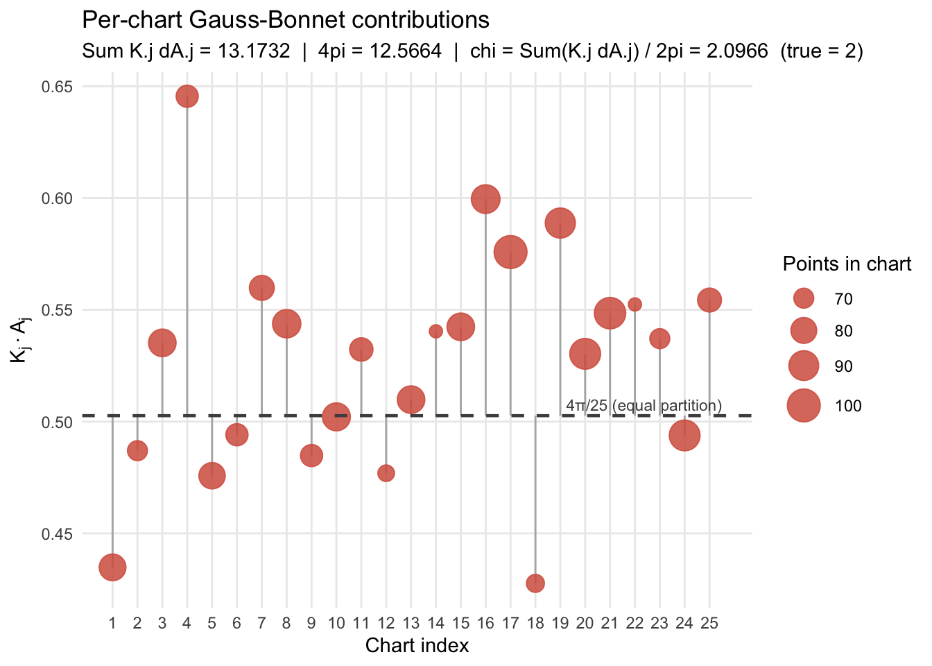
The following charts shows the results of the per chart calculations of the product \(K_i dA_i\) for each of the twenty-five charts.
The ~5% residual in \(\iint K\,dA\) has two equal contributors:
Curvature overestimate (\(\bar{K} \approx 1.05\)): the quadratic chart map approximates the sphere to second order; the small residual in the normal-direction fit inflates \(\det(\mathrm{II})\) slightly.
Area overestimate (\(\hat{A} / 4\pi \approx 1.01\)): the \(k\)-NN estimator has a mild positive bias at finite sample size \(N = 2000\).
Both biases are finite-sample effects that shrink as \(N \to \infty\) — they do not reflect a systematic geometric error in the atlas. The recovered Euler characteristic \(\chi \approx 2\) is fully consistent with the topological type of \(S^2\).
Summary
This post provides an R implementation of the Atas-Learn algorithm of Robinett et al. demonstrates that the algorithm provides close approximations to the theoretical results for the known case of the two dimensional sphere \(S^2\) in \(\mathbb{R^3}\). The validation tests performed were.
Geodesic fidelity: the atlas geodesic traces a full great circle with bounded deviation from the analytic path. On-manifold drift oscillates near zero across chart transitions, confirming that quasi-Euclidean steps do not systematically leave \(S^2\).
Constant curvature: every chart independently estimates \(K \approx 1\) and \(R \approx 1\).
Gauss-Bonnet Theorem: integrating per-point curvature weighted by atlas-derived area elements recovers Euler characteristic \(\chi \approx 2\) which is the the topological fingerprint of \(S^2\).
Together these results provide data-driven evidence that the Atlas-Learn algorithm learns the unit sphere to a close approximation.
References
[1] Robbin, Joel W.; Salamon, Dietmar A. (2022). Introduction to Differential Geometry (Springer Studium Mathematik (Master)) (p. 10). (Function). Kindle Edition.
[2] Robinett, R. A., Madejski, S. A., Ruark, K., Riesenfeld, S. J., & Orecchia, L. (2025). Atlas-based manifold representations for interpretable Riemannian machine learning. arXiv:2510.17772. Code repository: https://anonymous.4open.science/r/atlas_graph_learning-6DE0.
Appendix: Geodesic Integration via Quasi-Euclidean Retraction
Pullbacks vs. Exponential Maps
The canonical Riemannian tool for geodesic integration is the exponential map\(\exp_p : T_p\mathcal{M} \to \mathcal{M}\), which maps a tangent vector \(v \in T_p\mathcal{M}\) to the point reached by following the unique geodesic through \(p\) with initial velocity \(v\) for unit time. Computing \(\exp_p\) exactly requires solving the geodesic ODE:
where \(\Gamma^k_{ij}\) are the Christoffel symbols of the Levi-Civita connection, themselves derived from second derivatives of the metric tensor. On a manifold known only through a finite point cloud, neither the metric nor its derivatives are available in closed form, so computing Christoffel symbols directly is not feasible.
Atlas-Learn avoids this by using the chart Jacobian \(J_j(\xi)\) as a pullback of the ambient Euclidean structure. The inverse chart map \(\varphi_j^{-1} : \mathbb{R}^2 \to \mathbb{R}^3\) induces a pullback metric (the first fundamental form) on the chart domain:
where \((g_j)_{ab} = \sum_{i=1}^3 \partial_a(\varphi_j^{-1})_i\,\partial_b(\varphi_j^{-1})_i\). This is the metric that measures lengths and angles on\(\mathcal{M}\) as seen through the chart. The Moore–Penrose pseudoinverse:
is then the metric dual of \(J_j\): it pulls an ambient displacement \(\delta x \in \mathbb{R}^3\) back to the chart-coordinate displacement \(\delta\xi = J_j^+\,\delta x\) that minimizes \(\|\delta x - J_j\,\delta\xi\|^2\), i.e. the orthogonal projection of \(\delta x\) onto the tangent plane \(T_{x_t}\mathcal{M}\). The composition \(J_j J_j^+ = P_{T}\) is precisely the orthogonal projector onto \(T_{x_t}\mathcal{M}\), while \(J_j^+ J_j = I_2\) (within a single chart), confirming that a round-trip pullback–pushforward is exact.
Each retraction step therefore implements a first-order approximation to \(\exp_{x_t}\) using only quantities already computed during the atlas construction — no Christoffel symbols, no ODE solver.
The Transported Vector
The object that is propagated along the curve is the chart-coordinate velocity\(\tau \in \mathbb{R}^2\), a fixed-length 2-vector representing the initial direction in the tangent plane of the host chart. At every step it is pushed forward to an ambient direction by
applied as the retraction step, and then the Jacobian is recomputed at the new position \(\xi_{t+1}\). Keeping \(\tau\) fixed while updating \(J\) is an identity-transport approximation: the components of the velocity vector in the local frame are held constant rather than being corrected for the rotation of the frame as it moves. For a flat surface this is exact. For a curved surface like \(S^2\) it incurs an \(O(\varepsilon^2)\) error per step (where \(\varepsilon\) is the step size) because it omits the connection correction \(-\Gamma^k_{ij}\,\dot\gamma^i\,\dot\gamma^j\,\varepsilon\) that genuine parallel transport would apply. Over \(N \sim 1/\varepsilon\) steps the accumulated deviation is \(O(\varepsilon)\), which shrinks as the step size is reduced.
Why the Jacobian Update Approximates a Geodesic
A curve \(\gamma(t)\) on \(\mathcal{M}\) is a geodesic if and only if its velocity \(\dot\gamma\) is parallel transported along itself — that is, the covariant derivative \(\nabla_{\dot\gamma}\dot\gamma = 0\). In local chart coordinates this is exactly the geodesic ODE with Christoffel symbol corrections.
In Atlas-Learn the curvature of the surface is captured by the quadratic term\(m_j K_j \phi(\xi)\) in the chart map, which causes \(J_j(\xi)\) to vary smoothly with \(\xi\). At each step the algorithm:
Computes the ambient step \(J_j(\xi_t)\,\tau\) — using the current Jacobian to push the constant chart-velocity into the correct tangent plane at \(x_t\).
Pulls back the resulting ambient point \(x_{t+1}\) into chart coordinates via \(J_j^+\), keeping the curve on the learned surface.
Re-evaluates \(J_j\) at \(\xi_{t+1}\), so the tangent plane for the next step is the one at \(x_{t+1}\), not \(x_t\).
Step 3 is the key: updating \(J\) at each iteration implicitly steers \(\tau\) to remain in the tangent plane of the current point. This is a discretized version of the condition \(\dot\gamma \in T_{\gamma(t)}\mathcal{M}\) for all \(t\), which, combined with the unit-speed normalization of \(\tau\), gives a curve that approximates a geodesic to first order in \(\varepsilon\). The approximation becomes the true geodesic in the limit \(\varepsilon \to 0\), assuming the chart maps converge to the true surface.
The Retraction Loop
Concretely, each step of the integration proceeds as follows:
Identify the host chart \(j\) for \(x_t\), with local coordinates \(\xi_t = L_j^\top(x_t - \bar{x}_j)\).
Advance in chart coordinates using the pseudoinverse: \[\xi_{t+1} = \xi_t + J_j^+(\xi_t)\;(\varepsilon\,u_t), \qquad
J_j^+(\xi) = \bigl(J_j^\top J_j\bigr)^{-1}J_j^\top.\]
Evaluate the new ambient position: \(x_{t+1} = \varphi_j^{-1}(\xi_{t+1})\).
If \(\xi_{t+1} \notin \Omega_j\), locate the nearest valid chart \(j'\) and re-project: \(\xi_{t+1} \leftarrow L_{j'}^\top(x_{t+1} - \bar{x}_{j'})\).
Update the Jacobian: \(J \leftarrow J_{j'}(\xi_{t+1})\).
For the unit sphere \(S^2\) the true geodesics are great circles, providing a ground truth against which to measure the accumulated retraction error.